Caner Ozdemir - Inverse Synthetic Aperture Radar Imaging With MATLAB Algorithms

(2.75)

Putting Eq. 2.75into 2.72, one can get

(2.76)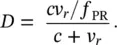

The new PRF for the reflected pulse is

(2.77)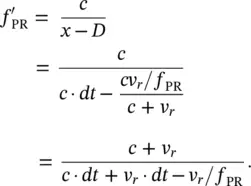

Substituting Eq. 2.75to the above equation, one can get the relationship between the PRFs of incident and reflected waves as

(2.78)

If the center frequency of the incident and reflected waves are f 0and , these two frequencies are related to each other with the same factor:

(2.79)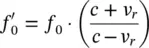

To find the Doppler shift in the frequency, f D, we should subtract the center frequency of the incident wave from the center frequency of the reflected wave as

(2.80)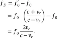

Since it is also obvious that the target velocity is very small compared to the speed of light (i.e. v r≪ c ), Eq. 2.81simplifies as

(2.81)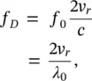

where λ 0is the wavelength corresponding to the center frequency of f 0. For the target that is moving away from the radar, the Doppler frequency shift has a negative sign as

(2.82)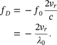

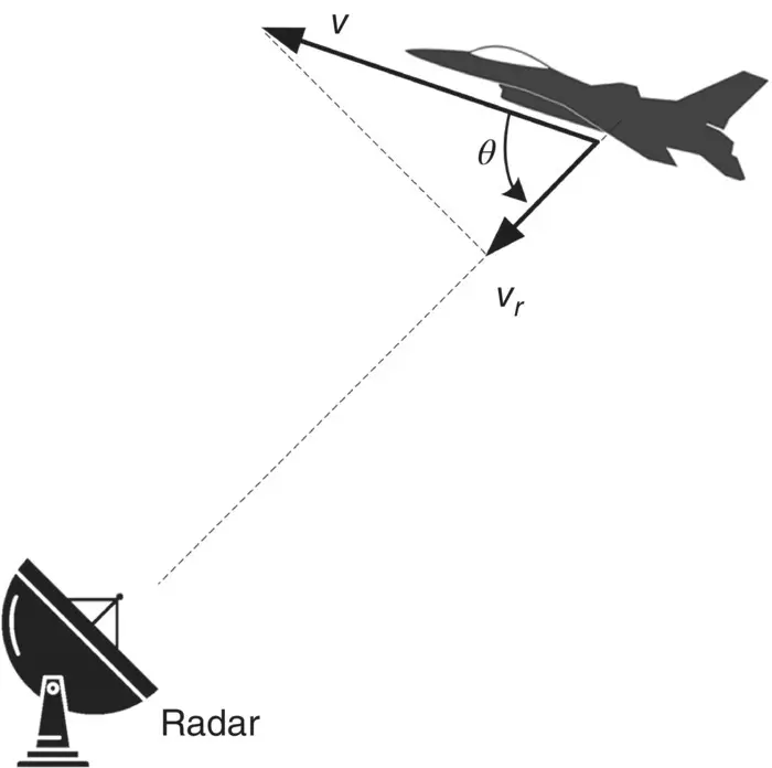
Figure 2.23 Doppler shift is caused by the target's radial velocity, v r.

It is clear from these equations that Doppler frequency shift is directly proportional to the velocity of the target. If the velocity increases, the shift in the frequency increases as well. If the target is stationary with respect to radar ( v r= 0), then the Doppler frequency shift is zero. The velocity v rin the above equation corresponds to the velocity along the RLOS direction. If the target is moving along another direction, v rrefers to the velocity projected toward the direction of radar. If the target's velocity is v as illustrated in Figure 2.23, then the Doppler frequency shift in terms of the target's original velocity will be equal to

(2.83)

Below are the Matlab source codes that were used to generate all of the Matlab‐produced figures in this chapter. The codes are also provided in the CD that accompanies this book.

%--------------------------------------------------------- % This code can be used to generate Figure 2.9%--------------------------------------------------------- %--- Figure 2.9a--------------------------------------------- clear close all fo=1e3; % set the frequency t=-4e-3:1e-7:4e-3; % choose time vector s=cos(2*pi*fo*t); % time domain CW signal plot(t*1e3,s,'k','LineWidth',2); grid minor set(gca,'FontName', 'Arial', 'FontSize',12,'FontWeight','Bold'); xlabel('\ittime, ms'); ylabel('\itamplitude, V'); axis([-4 4 -1.2 1.2]) %--- Figure 2.9(b)------------------------------------------- N=length(t); df=1/(t(N)-t(1)); % Find frequency resolution f=-df*(N-1)/2:df:df*(N-1)/2; % set frequency vector figure; S=fft(s)/N; % frequency domain CW signal plot(f*1e-3,fftshift(abs(S)),'k','LineWidth',2); grid minor set(gca,'FontName', 'Arial', 'FontSize',12,'FontWeight','Bold'); xlabel('\itfrequency, KHz'); ylabel('\itamplitude, V'); axis([-.8e1 .8e1 0 .6])

%-------------------------------------------------------- % This code can be used to generate Figure 2.11%-------------------------------------------------------- clear close all fo=100; % set the base frequency t=0:1e-7:4e-3; % choose time vector k=3e6; % select chirp rate m=sin(2*pi*(fo+k*t/2).*t); % time domain FMCW signal plot(t*1e3,m,'k','LineWidth',2); grid minor set(gca,'FontName', 'Arial', 'FontSize',12,'FontWeight','Bold'); xlabel('\ittime, ms'); ylabel('\itamplitude, V'); axis([0 4 -1.1 1.1])

%-------------------------------------------------------- % This code can be used to generate Figure 2.15%-------------------------------------------------------- clear close all c=.3; % speed of light [] f=2:.002:22; % choose frequency vector Ro=50; % choose range of target [m] k=2*pi*f/c; Es=1*exp(-1i*2*k*Ro); % collected SFCW electric field df=f(2)-f(1); % frequency resolution N=length(f); % total stepped frequency points dr=c/(2*N*df); % range resolution R=0:dr:dr*(length(f)-1); %set the range vector plot(R, 20*log10(abs(ifft(Es))),'k','LineWidth',2) grid minor set(gca,'FontName', 'Arial', 'FontSize',12,'FontWeight','Bold'); xlabel('\itrange, m'); ylabel('\itamplitude, dBsm'); axis([0 max(R) -90 0])

%--------------------------------------------------------- % This code can be used to generate Figure 2.16%--------------------------------------------------------- clear close all t=0:0.01e-9:50e-9; % choose time vector N=length(t); pulse(201:300)=ones(1,100); % form rectangular pulse pulse(N)=0; % Frequency domain equivalent dt=t(2)-t(1); % time resolution df=1/(N*dt); % frequency resolution f=0:df:df*(N-1); % set frequency vector pulseF=fft(pulse)/N; % frequency domain signal %--- Figure 2.16(a)------------------------------------------ plot(t(1:501)*1e9,pulse(1:501),'k','LineWidth',2); grid minor set(gca,'FontName', 'Arial', 'FontSize',12,'FontWeight','Bold'); xlabel('\ittime, ns'); ylabel('\itamplitude, V'); axis([0 5 0 1.1]); %--- Figure 2.16(b)------------------------------------------ figure plot(f(1:750)/1e9,20*log10(abs(pulseF (1:750))),'k','LineWidth',2); grid minor set(gca,'FontName', 'Arial', 'FontSize',12,'FontWeight','Bold'); axis([0 f(750)/1e9 -85 -20]); xlabel('\itfrequency, GHz'); ylabel('\itamplitude, dB');

%--------------------------------------------------------- % This code can be used to generate Figure 2.17%--------------------------------------------------------- clear close all t=-25e-9:0.01e-9:25e-9; % choose time vector N=length(t); sine(2451:2551)=-sin(2*pi*1e9*(t(2451:2551))); % form sine pulse sine(N)=0; % Frequency domain equivalent dt=t(2)-t(1); % time resolution df=1/(N*dt); % frequency resolution f=0:df:df*(N-1); % set frequency vector sineF=fft(sine)/N; % frequency domain signal %--- Figure 2.17(a)------------------------------------------------ plot(t(2251:2751)*1e9,sine (2251:2751),'k','LineWidth',2); grid minor set(gca,'FontName', 'Arial', 'FontSize',12,'FontWeight','Bold'); xlabel('\ittime, ns'); ylabel('\itamplitude, V'); axis([-2.5 2.5 -1.1 1.1]); %--- Figure 2.17(b)------------------------------------------------ figure plot(f(1:750)/1e9,20*log10(abs(sineF (1:750))),'k','LineWidth',2); grid minor set(gca,'FontName', 'Arial', 'FontSize',12,'FontWeight','Bold'); axis([0 f(750)/1e9 -85 -20]); xlabel('\itfrequency, GHz'); ylabel('\itamplitude, dB');