Caner Ozdemir - Inverse Synthetic Aperture Radar Imaging With MATLAB Algorithms

As pulses are repeated in T PR, the corresponding PRF of the radar is as given in Eq. 2.60. PRF gives the total number of pulses transmitted in every second by the radar. In radar applications, PRF value can be quite critical as it is linked to maximum range of a target, R max, and the maximum Doppler frequency, f D,max(so the maximum target velocity v maxof the target), that can be detectable by the radar. The use of PRF in ISAR range‐Doppler processing will be explored in Chapter 6.

As calculated in Eq. 2.58. the range resolution is proportional to the pulse duration as Δ r = c · τ /2. Therefore, the smaller the pulse duration, the finer the range resolution we can get. On the other hand, maximum range is determined by time delay between the transmitted and received pulses. Since the pulses are repeated for every T PRseconds, any received pulse that is reflected back from a target at R distant on the range should arrive before the next pulse is transmitted to avoid the ambiguity in the range, that is,

(2.63)

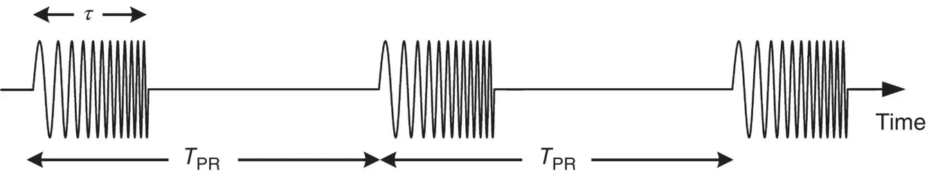
Figure 2.21 Pulsed radar systems use a sequence of modulated pulses.

If T PRis fixed, then the range should be less than the following quantity:

(2.64)

Therefore, the maximum range that can be unambiguously detected by the pulsed radar is calculated by the period between the pulses, that is, T PR, as given below:

(2.65)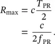

This is also called unambiguous range since any target within this range is accurately detected by the radar at its true location. However, any target beyond this range will be dislocated in the range as the radar can only display the R maxmodulus of the target's location along the range axis. To resolve the range ambiguity problem, some radars use multiple PRFs while transmitting the pulses (Mahafza 2005).

In radar theory, the concept of Doppler frequency describes the shift in the center frequency of an incident EM wave due to movement of radar with respect to target. The basic concept of Doppler shift in frequency has been conceptually demonstrated through Figure 2.10and is defined as

(2.66)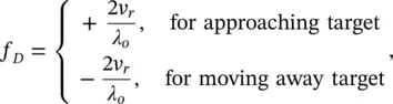

where v ris the radial velocity along the radar line of sight (RLOS) direction. Now, we will demonstrate how the shift in the phase (also in the frequency) of the reflected signal from a moving target constitutes. Let us consider an object moving toward the radar with a speed of v r. The radar produces and sends out pulses with the PRF value of f PR. Every pulse has a time duration (or width) of τ . The illustration of Doppler frequency shift phenomenon is given in Figure 2.22. The leading edge of the first pulse hits the target (see Figure 2.22a). After a time advance of Δ t . the trailing edge of the first pulse hits the target as shown in Figure 2.22b. During this time period, the target traveled a distance of

(2.67)

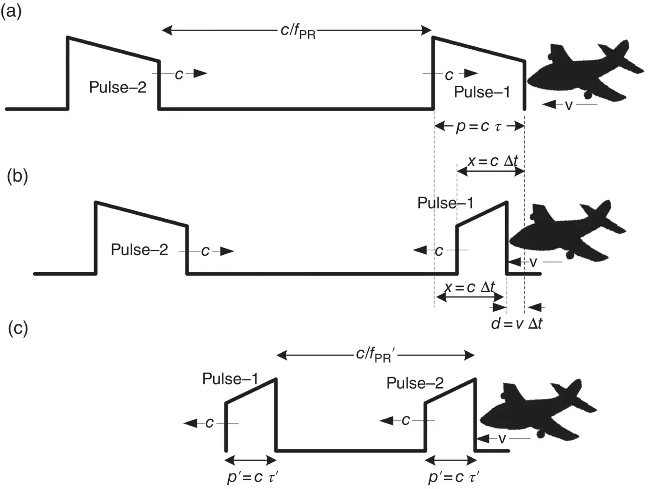
Figure 2.22 Illustration of Doppler shift phenomenon: (a) the leading edge of the first pulse in hitting the target at t = 0; (b) the trailing edge of the first pulse in hitting the target at t = Δ t ; (c) the trailing edge of the second pulse is hitting the target at t = dt . During this period, the target traveled a distance of D = v r× dt .

Looking at the situation in Figure 2.22b, it is obvious that the pulse distance before the reflection is equal to the distance traveled by the leading (or trailing) edge of the pulse plus the distance traveled by the target as

(2.68)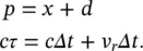

Similarly, the pulse distance after the reflection is equal to the distance traveled by the leading (or trailing) edge of the pulse minus the distance traveled by the target as

(2.69)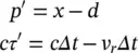

Dividing these last two equations yields

(2.70)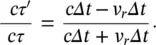

On the left‐hand side of this equation, c terms are canceled, whereas Δ t terms are canceled on the right‐hand side. Then, the pulse width after the reflection can be written in terms of the original pulse width as

(2.71)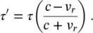

The term ( c − v r)/( c + v r) is known as the dilation factor in the radar community. Notice that when the target is stationary ( v r= 0), then the pulse duration remains unchanged ( τ ' = τ ) as expected.

Now, consider the situation in Figure 2.22c. As trailing edge of the second pulse is hitting the target, the target has traveled a distance of

(2.72)

within the time frame of dt . During this period, the leading edge of the first pulse has traveled a distance of

(2.73)

On the other hand, the leading edge of the second pulse has to travel a distance of ( c / f PR− D ) at the instant when it reaches the target. Therefore,

(2.74)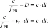

Solving for dt yields