Caner Ozdemir - Inverse Synthetic Aperture Radar Imaging With MATLAB Algorithms
Здесь есть возможность читать онлайн «Caner Ozdemir - Inverse Synthetic Aperture Radar Imaging With MATLAB Algorithms» — ознакомительный отрывок электронной книги совершенно бесплатно, а после прочтения отрывка купить полную версию. В некоторых случаях можно слушать аудио, скачать через торрент в формате fb2 и присутствует краткое содержание. Жанр: unrecognised, на английском языке. Описание произведения, (предисловие) а так же отзывы посетителей доступны на портале библиотеки ЛибКат.
- Название:Inverse Synthetic Aperture Radar Imaging With MATLAB Algorithms
- Автор:
- Жанр:
- Год:неизвестен
- ISBN:нет данных
- Рейтинг книги:5 / 5. Голосов: 1
-
Избранное:Добавить в избранное
- Отзывы:
-
Ваша оценка:
Inverse Synthetic Aperture Radar Imaging With MATLAB Algorithms: краткое содержание, описание и аннотация
Предлагаем к чтению аннотацию, описание, краткое содержание или предисловие (зависит от того, что написал сам автор книги «Inverse Synthetic Aperture Radar Imaging With MATLAB Algorithms»). Если вы не нашли необходимую информацию о книге — напишите в комментариях, мы постараемся отыскать её.
covers in greater detail the fundamental and advanced topics necessary for a complete understanding of inverse synthetic aperture radar (ISAR) imaging and its concepts. Distinguished author and academician, Caner Özdemir, describes the practical aspects of ISAR imaging and presents illustrative examples of the radar signal processing algorithms used for ISAR imaging. The topics in each chapter are supplemented with MATLAB codes to assist readers in better understanding each of the principles discussed within the book.
This new edition incudes discussions of the most up-to-date topics to arise in the field of ISAR imaging and ISAR hardware design. The book provides a comprehensive analysis of advanced techniques like Fourier-based radar imaging algorithms, and motion compensation techniques along with radar fundamentals for readers new to the subject.
The author covers a wide variety of topics, including:
Radar fundamentals, including concepts like radar cross section, maximum detectable range, frequency modulated continuous wave, and doppler frequency and pulsed radar The theoretical and practical aspects of signal processing algorithms used in ISAR imaging The numeric implementation of all necessary algorithms in MATLAB ISAR hardware, emerging topics on SAR/ISAR focusing algorithms such as bistatic ISAR imaging, polarimetric ISAR imaging, and near-field ISAR imaging, Applications of SAR/ISAR imaging techniques to other radar imaging problems such as thru-the-wall radar imaging and ground-penetrating radar imaging Perfect for graduate students in the fields of electrical and electronics engineering, electromagnetism, imaging radar, and physics,
also belongs on the bookshelves of practicing researchers in the related areas looking for a useful resource to assist them in their day-to-day professional work.
Inverse Synthetic Aperture Radar Imaging With MATLAB Algorithms — читать онлайн ознакомительный отрывок
Ниже представлен текст книги, разбитый по страницам. Система сохранения места последней прочитанной страницы, позволяет с удобством читать онлайн бесплатно книгу «Inverse Synthetic Aperture Radar Imaging With MATLAB Algorithms», без необходимости каждый раз заново искать на чём Вы остановились. Поставьте закладку, и сможете в любой момент перейти на страницу, на которой закончили чтение.
Интервал:
Закладка:
(2.28) 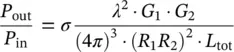
In this equation, L totis the total loss accounted for all the losses and is given by
(2.29) 
If both the transmitter and the receiver antenna are perfectly matched and there are no losses inside the transmission lines, then L tot= 1; therefore, Eq. 2.28can be simplified to give
(2.30) 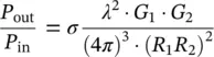
2.4.2 Monostatic Case
In the case of monostatic operation of radar, the same antenna is used for transmitting the radar signal and receiving the backscattered wave from the target (see Figure 2.7). Therefore, the antenna gains, G 1and G 2in Eq. 2.30, become identical, say G (= G 1= G 2). Similarly, the target distance from the transmitter and the receiver distance from the target becomes equal, say R (= R 1= R 2). Then the radar range equation can be obtained in its simplified form as shown below:
Figure 2.7 Geometry for obtaining monostatic radar range equation.
(2.31) 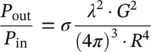
2.5 Range of Radar Detection
While working with radars, another important parameter that should be carefully considered is the detection range of radar, that is, the farthest distance of the target that can be detected over the noise floor of the radar. This distance can be easily calculated starting from the radar range equation. Let us rewrite Eq. 2.31in terms of antenna effective aperture, A eff= 4 π ⋅ G 2/ λ 2, as
(2.32) 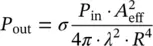
The minimum power at the receiver output can only be detected if the received signal is greater than the noise floor, as demonstrated in Figure 2.8. If the power level at the receiver output is lower than the noise floor, this signal cannot be distinguished from the noise mostly produced by the environment and the electronic equipment and therefore can either be considered as noise or clutter.
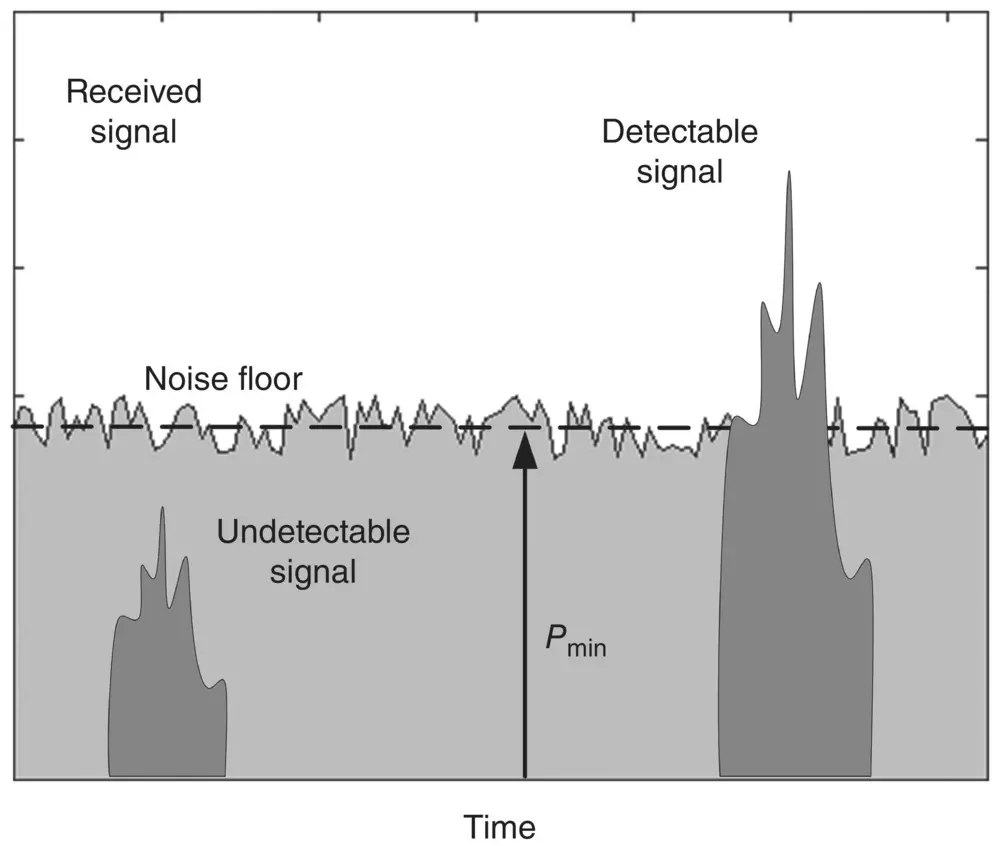
Figure 2.8 Minimum receiver power corresponding to maximum range of radar.
Considering that the input power to the radar remains unchanged, the output power at the receiver in Eq. 2.32is selected as the minimum detectable signal, P min, for the maximum range distance of R maxas
(2.33) 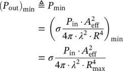
Therefore, it is easy to find the maximum range of radar by rearranging the above equation to leave R maxalone as
(2.34) 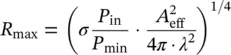
The above equation gives the maximum range of an object that can be detectable by the radar. The meaning of “maximum range” is clarified with the following example: For a radar antenna with 26 dB gain at 10 GHz, the corresponding antenna effective area becomes 28 472 m 2. If the input power of this monostatic radar is 75 W with a receiver sensitivity of −55 dBmW (3.16 nW) and used to detect a target with an RCS of 0.5 m 2at 10 GHz, then the maximum range can be readily calculated by plugging the appropriate numbers into above equation to give
(2.35) 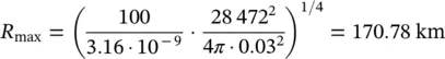
If this target is located at the range closer than 170.78 km (~171 km), then it will be detected by this radar. However, any object that has a maximum RCS of 0.5 m 2and located beyond 171 km will not be perceived as a target since the received signal level will be lower than the sensitivity level (or the noise floor) of the radar as illustrated in Figure 2.8.
2.5.1 Signal‐to‐Noise Ratio
Similar to all electronic devices and systems, radars must function in the presence of internal noise and external noise. The main source of internal noise is the agitation of electrons caused by heat. The heat inside the electronic equipment can also be caused by environmental sources such as the sun, the earth, and buildings. This type of noise is also known as thermal noise (Johnson 1928) in the electrical engineering community.
Let us investigate the signal‐to‐noise ratio (SNR) of a radar system: Similar to all electronic systems, the noise power spectral density of a radar system can be described as the following equation:
(2.36) 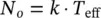
Here, k = 1.381 × 10 −23W/K° is the well‐known Boltzman constant, and T effis the effective noise temperature of the radar in degrees Kelvin (K°). T effis not the actual temperature but is related to the reference temperature via the noise figure , F n, of the radar as
(2.37) 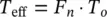
where the reference temperature, T o, is usually referred to as room temperature ( T o≈ 290 K°). Therefore, noise power spectral density of the radar is then being equated to
(2.38) 
To find the value of the noise power , P n, of the radar, it is necessary to multiply N owith the effective noise bandwidth , B n, of the radar as shown below:
(2.39) 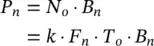
Here, B nmay not be the actual bandwidth of the radar pulse; it may extend to the bandwidth of the other electronic components such as the matched filter at the receiver. Provided that the noise power is determined, it is easy to define the SNR of radar by combining Eqs. 2.28and 2.39as below:
Читать дальшеИнтервал:
Закладка:
Похожие книги на «Inverse Synthetic Aperture Radar Imaging With MATLAB Algorithms»
Представляем Вашему вниманию похожие книги на «Inverse Synthetic Aperture Radar Imaging With MATLAB Algorithms» списком для выбора. Мы отобрали схожую по названию и смыслу литературу в надежде предоставить читателям больше вариантов отыскать новые, интересные, ещё непрочитанные произведения.


Обсуждение, отзывы о книге «Inverse Synthetic Aperture Radar Imaging With MATLAB Algorithms» и просто собственные мнения читателей. Оставьте ваши комментарии, напишите, что Вы думаете о произведении, его смысле или главных героях. Укажите что конкретно понравилось, а что нет, и почему Вы так считаете.