Andrea Vacca - Hydraulic Fluid Power

Find:

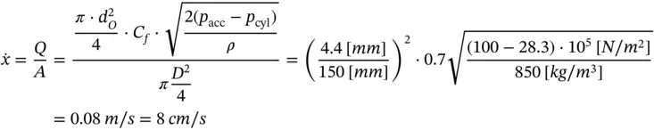
The extension velocity of the piston,

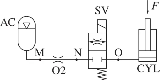
The system contains a solenoid valve (SV; which will be further described in Chapter 8), which when energized opens an accumulator to the piston chamber of a linear accumulator. For simplicity, the accumulator can be seen as a constant pressure source. In reality, the pressure inside the accumulator will decrease as the accumulator releases flow, as it will be better described in Chapter 9.

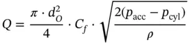
When the valve is energized, the flow rate across it is defined by the orifice equation:

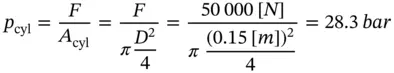
The pressure inside the cylinder is given by the external force:

Therefore, the actuator speed is

In order to reduce the actuator's speed, there are possible alternatives:

1 Increase the piston diameter.

2 Decrease the valve size, thus reducing the valve coefficient k.

3 Reduce the accumulator pressure.

4 Add an orifice in series with the valve (see figure below).

All mentioned solutions are reasonable; however, solutions 1, 2, and 3 require modifications to the existing components. Solution 4 can be a simple way to modify an existing system.

The flow rate through the orifice and the valve can be written as

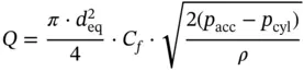
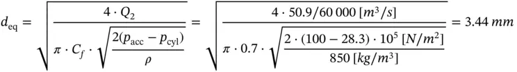
d eqis the diameter of the equivalent orifice given by the series connection of SV and O2. The desired speed of the actuator corresponds to the following flow:

The equivalent series orifice diameter results:

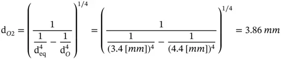
Assuming that both orifices have the same flow coefficient ( C f= 0.7), the diameter of orifice O2 results:

Even though the orifice element is described by a single equation ( Eq. (4.5)), an orifice can assume different roles in a hydraulic circuit. A first way to classify an orifice function is based on its location in the system: in fact, orifices can be present either in the working and return lines or on the pilot lines of the systems. The working and return lines are represented by the connections to/from the actuators of the system; the power transfer functions achieved by the system occur in these lines. Thus, these lines are usually characterized by significant values of flow rate and pressure. Pilot lines are instead used to transmit pressure information to different locations of the system. These latter lines usually have negligible flow rates and are used for control purposes. According to ISO1219‐1 [1], pilot lines are always indicated with dashed lines, while working and return lines with a solid line.

When an orifice is used in the working or the return line of a system, it can operate as metering or compensating element.

In principle, if an orifice establishes the flow rate, for a given pressure drop, it functions as a metering element; however, if the orifice defines a certain pressure drop for a given flow rate, it functions as a compensator. In both cases, the relation between pressure drop and flow rate across the orifice is given by Eq. (4.5).

This classification is important to understand several control strategies used in hydraulic systems, as it will be shown in Part IIand Part IIIof the book. A significant example is now provided to clarify the distinction between these different behaviors of an orifice.

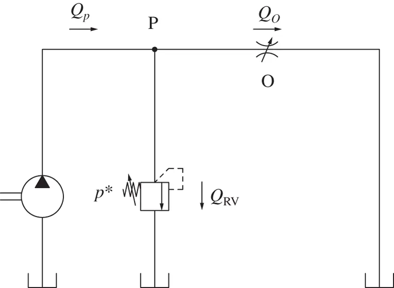
The system in figure consists of a fixed displacement pump and a variable orifice in parallel with a pressure relief valve. The pressure relief valve limits the maximum pressure at the pump outlet to p* . The pump delivers a fixed flow rate Q Pindependently of the pump outlet pressure. Find the flow rate through the orifice, Q O, as well as the pump outlet pressure p P, as a function of the orifice area opening, Ω. Describe also the function of the orifice, which can either be metering or compensator.

Given:

The pump flow rate, Q P; the setting of the relief valve p* .

Find:

1 The flow rate through the orifice, QO

2 The pressure at pump outlet, pP

3 The orifice function (metering/compensator)

Point P is located at the junction of the three main elements of the system (the pump, the relief valve, the variable orifice). Therefore, the operating pressure at point P can be found by intersecting the characteristics curves of these components, while also satisfying the constraints of maximum allowed pressure and available flow.

To clarify this statement, the characteristic curves of the three components in the (Δ p , Q ) chart are shown in the figure below. In particular,

the orifice characteristic curves are plotted according to the orifice equation 4.5for decreasing values of the area Ω (Ω1 > Ω2 > Ω3…). This trend is as also shown in the plot of Figure 4.4. It is important to observe that, in this case, the pressure drop across the orifice equals pP, since the pressure downstream the orifice is pT = 0 bar.

the pump curve represented by a horizontal line (constant flow rate). In fact, for this problem the pump provides a constant flow independent on the system pressure.

the relief valve curve, represented by a vertical line. The relief valve, which will be explained more in detail in Chapter 8, limits the maximum pressure at the junction point P to p*.

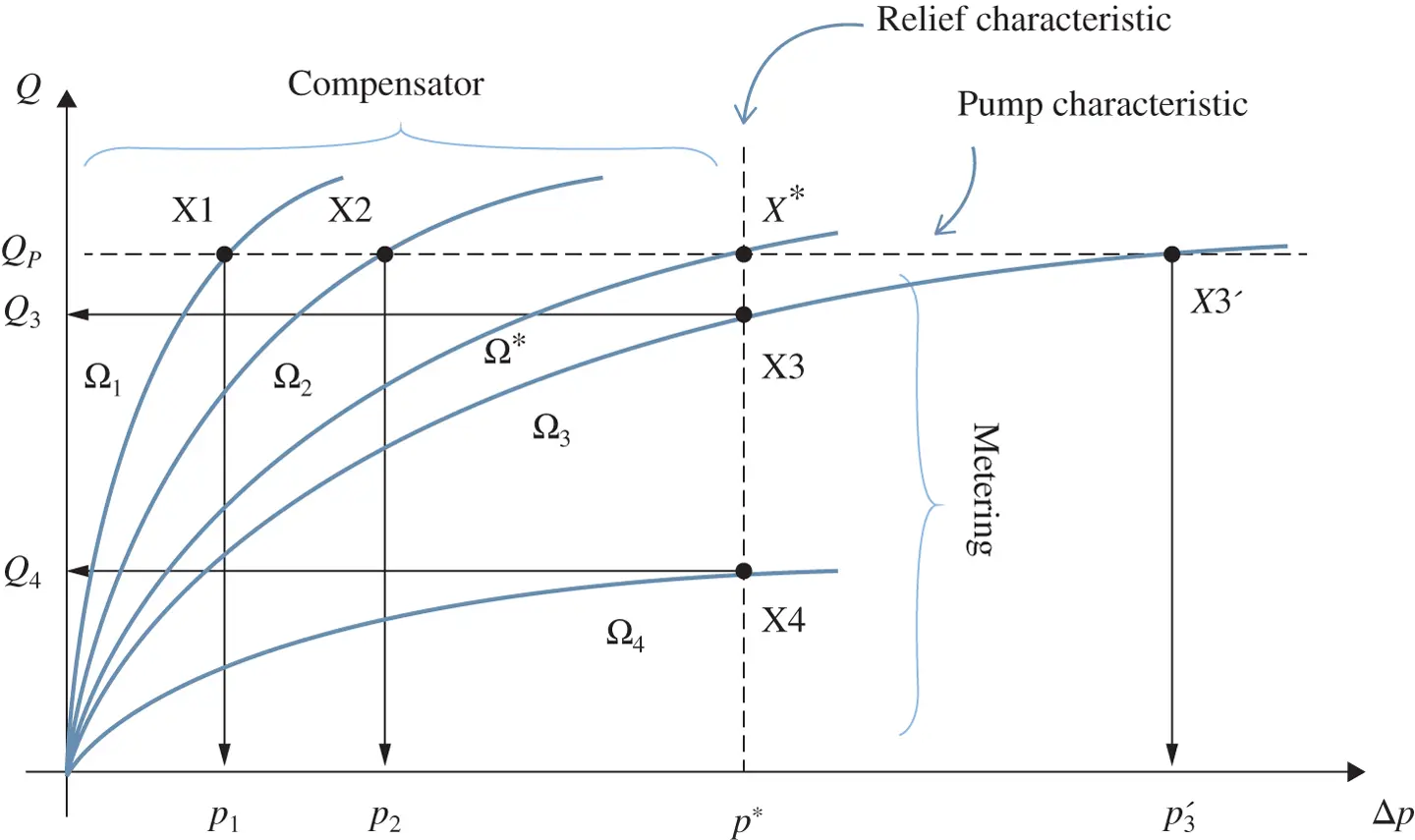
The behavior of the system can be analyzed for different openings of the variable orifice O.

In case of a large orifice area (Ω = Ω 1), the intersection between the pump characteristic and the orifice curve is at X1. This point is located at a pressure lower than p* : the entire pump flow rates Q Pgoes to the orifice ( Q P= Q O); and the relief valve is closed ( Q RV= 0). In this case, the orifice Eq. (4.5)can be used to find the pressure at the point P: