Andrea Vacca - Hydraulic Fluid Power

The coefficient of discharge not only is a pure geometrical ratio but also accounts for other secondary but non‐negligible aspects that affect the actual flow conditions through the orifice. These are the frictional effects due to fluid viscosity and the approximated flow uniformity. For these reasons, the empirical formulas available for C dshow a primary dependency of the coefficient of discharge with the Reynolds number. Empirical formulas for C dare available in the literature, such as in the Miller handbook [38] or the ASME standards [39].

The term 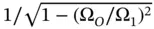is also referred to as the velocity of approach factor . Usually, the velocity of approach factor and the coefficient of discharge are combined in a single coefficient, often indicated as the flow coefficient or the orifice coefficient . Equation (4.4)then becomes 2

(4.5)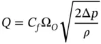

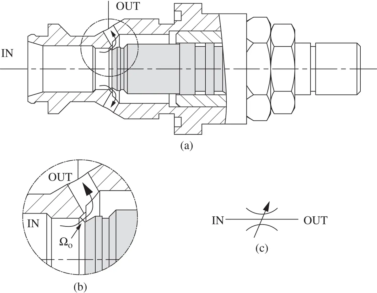
Figure 4.2 Orifice area for a poppet needle valve. (a) Entire popper valve. (b) Eetail on the throat flow area. (c) ISO symbol.

The same abovementioned references collected empirical formulas for the orifice coefficient for various geometries and sizes. In many cases, it can be simply assumed that Ω 1≫ Ω O: hence, the effects of velocity of approach are negligible and the value of C fcan be approximated with the coefficient of discharge C d.

The orifice equation has a very broad application in hydraulics because it can be used to describe the flow through any element of the system introducing one or more flow restrictions. Figure 4.2shows the example of a needle valve based on a poppet design. The orifice area Ω Ois represented by the minimum flow area and, in this case, it has an annular shape.

For any specific geometric case, the orifice coefficient should be determined experimentally. Several authors report the theoretical evaluation of such a coefficient for different geometries, under the assumptions of frictionless, incompressible and irrotational flow. For example, Von Mises [40] provided the analytical results for the flow coefficient for several different orifice geometries. A comparison between Von Mises' results and experimental data is also extensively discussed in [36].

As shown in [2, 32, 36], typical values for C fare in the range of 0.6–0.8. In particular, 0.611 is the von Mises' theoretical value for a circular sharp edge orifice ( Figure 4.1).

The value of the C fcoefficient can be considered constant only for high Reynolds numbers (turbulent flow conditions). In case of laminar flow, the flow through an orifice can be solved analytically from Navier‐Stokes equations. In the case of a circular sharp edge orifice, the relationship becomes [41]

(4.6)

Figure 4.3shows the trend for the C fcoefficient as a function of the Reynolds number, Re . In the figure, both theoretical solutions (Von Mises and Eq. (4.6)) are reported along with experimental results, as described in [36]. The measured trend for C fshows a smooth transition from the laminar behavior, typical of low fluid velocities, and the turbulent conditions. Qualitatively, the same trend represented in Figure 4.3applies to the orifice geometries and shape characteristics of common hydraulic control elements.

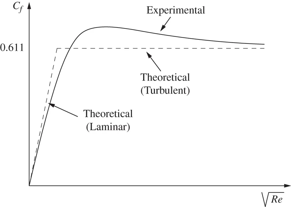
Figure 4.3 Theoretical and experimental trends of the flow coefficient vs. the Reynolds number.

The general orifice equation ( Eq. 4.5) shows how an orifice can be seen as a hydraulic resistance, according to the definition provided in Chapter 3( Eq. (3.38)):

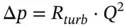
Therefore,

(4.7)

A fixed orifice is a hydraulic element characterized by a specific throat area Ω O; in a variable orifice , the area Ω Ocan vary according to the instantaneous geometric configuration.

Figure 4.2gives an example of a needle valve, which is an adjustable orifice. The characteristics of both fixed and variable orifices are represented in Figure 4.4. The relationship between pressure drop and flow rate for turbulent flow conditions is parabolic, and the curves show the trend for different orifice areas. The component working conditions pertain only to the first (positive flow) and the third quadrant (negative flow). The figure also highlights the symbols used to indicate both the fixed and the variable orifice cases.

It is important to remark the square root dependence between Δ p and Q highlighted in Figure 4.4. Because of this dependence, in order to double the flow across the orifice, it is necessary to increase the pressure by four times.

In hydraulic control valves, variable orifices are often used to represent the positions and the connections implemented by the valve. Figure 4.5shows the example of two proportional valves, one is a two‐position two‐way (a) and the other one is a three‐position four‐way (a). In both cases, each square represents the possible configurations of the port connections obtained by the valve, and the continuous lines above and below the symbols indicate that the orifice area of every connection can be continuously varied.

The valve symbol includes different details when compared to the representation with basic orifices. For instance, in Figure 4.5, the information about the closed configuration (all ports completely closed Ω O= 0) is not provided by the basic orifice symbols.

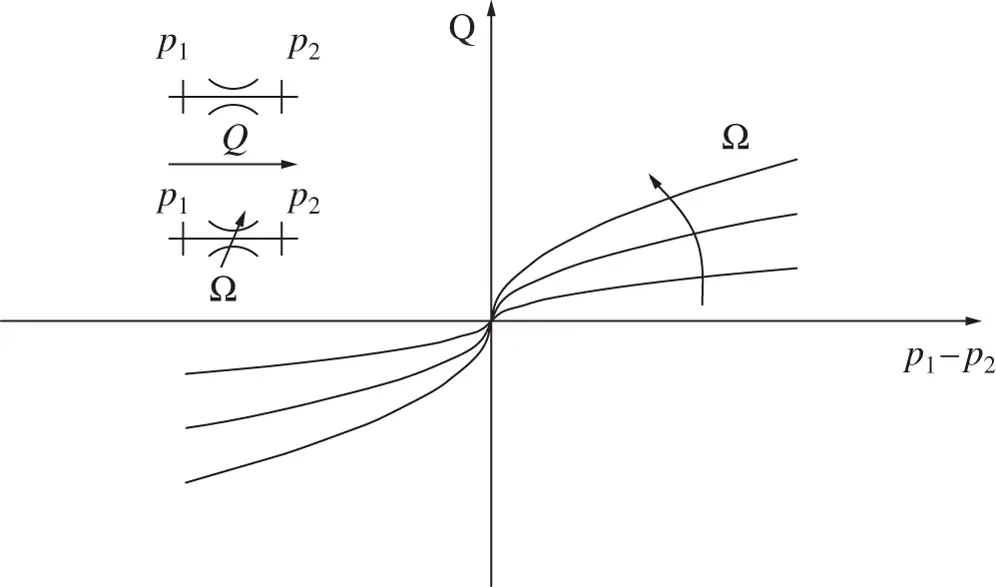
Figure 4.4 Orifice equation plotted in a (p, Q) layer for different area openings.

As explained in Chapter 3, the product Q · Δ p represents hydraulic power. For the case of an orifice, this product represents the power dissipation introduced by the orifice itself:

(4.8)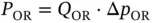

This power dissipation mostly goes into heat generation within the fluid. In most cases, the portion of heat exchange with the external environment (through the solid walls of the components in the system, including the orifice) is minimal and negligible. The temperature increase of the fluid can be calculated from the energy balance:

(4.9)