Andrea Vacca - Hydraulic Fluid Power
Здесь есть возможность читать онлайн «Andrea Vacca - Hydraulic Fluid Power» — ознакомительный отрывок электронной книги совершенно бесплатно, а после прочтения отрывка купить полную версию. В некоторых случаях можно слушать аудио, скачать через торрент в формате fb2 и присутствует краткое содержание. Жанр: unrecognised, на английском языке. Описание произведения, (предисловие) а так же отзывы посетителей доступны на портале библиотеки ЛибКат.

- Название:Hydraulic Fluid Power
- Автор:
- Жанр:
- Год:неизвестен
- ISBN:нет данных
- Рейтинг книги:3 / 5. Голосов: 1
-
Избранное:Добавить в избранное
- Отзывы:
-
Ваша оценка:
Hydraulic Fluid Power: краткое содержание, описание и аннотация
Предлагаем к чтению аннотацию, описание, краткое содержание или предисловие (зависит от того, что написал сам автор книги «Hydraulic Fluid Power»). Если вы не нашли необходимую информацию о книге — напишите в комментариях, мы постараемся отыскать её.
Readers of
will benefit from:
Approaching hydraulic fluid power concepts from an “outside-in” perspective, emphasizing a problem-solving orientation Abundant numerical examples and end-of-chapter problems designed to aid the reader in learning and retaining the material A balance between academic and practical content derived from the authors’ experience in both academia and industry Strong coverage of the fundamentals of hydraulic systems, including the equations and properties of hydraulic fluids
is perfect for undergraduate and graduate students of mechanical, agricultural, and aerospace engineering, as well as engineers designing hydraulic components, mobile machineries, or industrial systems.
Hydraulic Fluid Power — читать онлайн ознакомительный отрывок
Ниже представлен текст книги, разбитый по страницам. Система сохранения места последней прочитанной страницы, позволяет с удобством читать онлайн бесплатно книгу «Hydraulic Fluid Power», без необходимости каждый раз заново искать на чём Вы остановились. Поставьте закладку, и сможете в любой момент перейти на страницу, на которой закончили чтение.
Интервал:
Закладка:
4 3.4 A pumping system is used to fill an elevated hydraulic tank as shown in the figure below. The hose used has a 1.91‐cm (0.75 in.) diameter and 7.62‐m (25 ft) length. The internal roughness is 0.5 mm (1.97 10−2 in) and the gage pressure of the oil at the pump outlet is 379 kPa (55 psi). The oil density is 900 kg/m3 (62.4 lbm/ft3) and the viscosity of the oil is 4 10−6 m2/s (1.20 10−5 ft2/s).The minor loss coefficient due to the bends in the hose are much smaller than the minor loss coefficient due to the GV, positioned at the pump outlet. GV has a loss coefficient of 2. Determine the volumetric flow rate of the oil into the elevated tank.
5 3.5 Oil flows through two pipes with the same diameter, length, and friction factor. The flow rate through the second pipe is twice that through the first pipe. Both flows are turbulent and fully developed. Which statement is correct about the pressure drop over the pipe length, Δp, for the two pipes?Δp2 = 0.25Δp1Δp2 = 0.5Δp1Δp2 = Δp1Δp2 = 2Δp1Δp2 =4 Δp1
6 3.6 Oil of density 850 kg/m3 is flowing through the 180° elbow shown below. At the inlet of the elbow, the gage pressure is 1 bar. The oil discharges to the atmosphere. Assume properties are uniform over the inlet and outlet areas. Additionally, A1 = 25 cm2 and A2 = 2.5 cm2. The inlet velocity is 3.5 m/s. Find the horizontal component of the force to hold the elbow in place.
7 3.7 Water flows from a tank that sits on frictionless wheels. The pipe has a diameter of 0.5 m. The tank is open to atmospheric (location (1)) and it is connected with a 50‐m‐long pipe to a second pipe that is 75 m long, bolted at location (3). A filter with a loss coefficient K = 8 is placed along the second pipe and the flow exits to the atmosphere at location (2). All other minor losses are negligible.Use the generalized Bernoulli's equation to derive an expression for the velocity in the pipe as a function of the friction coefficient.Determine the pressure at the location (3), assuming a friction coefficient of 0.015.Use the CV approach and the momentum equation to determine the tension of the bolts of the flange at location (3).
8 3.8 A pump is used for a fountain jet as in the schematic shown in the figure below. The pump is connected to an electric motor that rotates at 1000 rpm. Following data for the system are given: D = 0.100 m; L = 1 m (L is the length of each branch, as shown in the figure); and relative roughness, /D = 0.02, for all pipe sections. The inlet of the pump is at the same elevation as the free surface of reservoir, as shown in the figure.Factors for minor losses are Kin = 0.5; Kbend = 1, Kconv= negligibleFor the water, assume ρ = 1000 kg/m3; μ = 1 × 10⁻³N s/m2Knowing that the pump characteristic curve is given by following equation:[Hp] = m, [Q] = m3/s, the units of the coefficients 10 and 625 are not written for convenience.Find the flow rate through the pump, in m3/s for Case A.Indicate the operating point of the system, in a (Q, H) plot (qualitative representation), for Case A.Find the elevation of the jet, Δh, in m, for Case A.Does the value of Δh increase/decrease, for the Case B? Calculate the Δh you get for Case B.Calculate the power requested by the electric motor.Assume the total efficiency of the pump η = 0.8.
Notes
1 1A significant exception to this statement is the analysis of suction conditions at the inlet of hydraulic pumps. Considerations on the suction ability of pumps as well as the occurrence of gaseous or vapor cavitation should be taken into account when determining the elevation of the reservoir with respect to the inlet port.
2 2In the literature, it also common to find the hydraulic resistance generally defined aswhich implies a linear relationship between flow rate and pressure drop. This will be the case of the laminar hydraulic resistance. In this book, the authors choose to distinguish the case of laminar hydraulic resistance from the case of turbulent hydraulic resistance.
3 3This is not exactly true for the exit section 2, as shown in the detail of the figure. However, it is usually a good approximation also because of the low velocity values that are typically present at the vena contraction.
Chapter 4 Orifice Basics
Flow restrictions such as orifices, flow nozzles, and venturis are known for introducing pressure losses associated with flow rate. In hydraulic control systems, the relationship between pressure drop and flow rate established by these restrictions (generally referred to as orifices) is the basis of the operating principle accomplished by most of the control elements in hydraulic systems, such as hydraulic control valves. Therefore, an entire chapter is dedicated to the orifice equation and its uses in hydraulic systems.
4.1 Orifice Equation
The orifice equation provides the relationship between the flow rate through a generic restriction and the pressure drop across it.
In this section, the orifice equation is derived for the particular case of a sharp orifice ( Figure 4.1). As shown in the figure, the internal flow is characterized by different phases. At first, the fluid stream accelerates approaching the restriction. Afterward, the flow separates from the sharp edge of the orifice, which causes recirculation zones downstream of the restriction. In this phase, the mainstream flow still continues to accelerate from the nozzle throat to form a vena contracta at section 2, where the flow area is minimum. The flow then decelerates to fill the duct section. At vena contracta, the flow streamlines are essentially straight, and the pressure is uniform across the section.
This flow condition can be well studied using the continuity and Bernoulli's equations. Then, empirical correction factors may be applied to estimate the correct flow rate, or to consider different geometrical conditions.
Under the assumption of incompressible flow, the mass conservation written between sections 1 and 2 of Figure 4.1gives
(4.1) 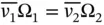
Bernoulli's equation applies to both sections 1 and 2 under the additional assumptions of stationary conditions, frictionless flow, and uniform velocities at each section 1 . Moreover, these sections are properly considered where no streamline curvature is present so that the pressure is uniform across the sections:
(4.2) 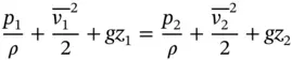
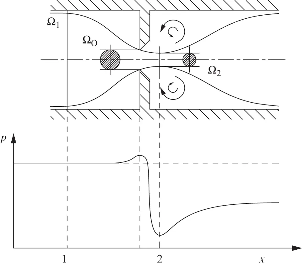
Figure 4.1 Flow through a sharp orifice.
The elevation term in Eq. (4.2)can be simplified by assuming z 1= z 2.
From Eqs. (4.1)and (4.2), it is possible to obtain the following expression for the volume flow rate Q = Q 1= Q 2:
(4.3) 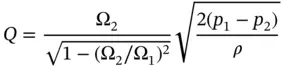
The actual flow area Ω 2in the vena contracta is unknown. Therefore, an empirical coefficient called the coefficient of discharge C dis introduced in order to write the equation referring to the known value Ω O:
(4.4) 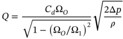
Интервал:
Закладка:
Похожие книги на «Hydraulic Fluid Power»
Представляем Вашему вниманию похожие книги на «Hydraulic Fluid Power» списком для выбора. Мы отобрали схожую по названию и смыслу литературу в надежде предоставить читателям больше вариантов отыскать новые, интересные, ещё непрочитанные произведения.


Обсуждение, отзывы о книге «Hydraulic Fluid Power» и просто собственные мнения читателей. Оставьте ваши комментарии, напишите, что Вы думаете о произведении, его смысле или главных героях. Укажите что конкретно понравилось, а что нет, и почему Вы так считаете.