Andrea Vacca - Hydraulic Fluid Power

The flow force F flcan be seen as the reaction force of the above F x, which is the force that the fluid exerts to the bounding surfaces of the CV.

(3.48)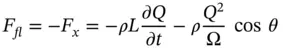

The flow force presents both a stationary component and a transient component. The stationary component corresponds to a given position of the spool or the poppet of the valve and a constant flow rate. The transient component relates to variations of the spool (or poppet) position, as well as flow variations. In typical problems, the transient component is neglected.

The first term refers to transient conditions, and it can be neglected when studying a stationary condition. Therefore, when studying hydraulic control valves, the second term, is normally the most important one.

(3.49)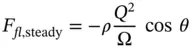

The negative sign in Eq. (3.48)implies that for the spool valve geometry of Figure 3.17, the flow force tends to reduce the opening area of the spool toward the outlet section 2. This is also qualitatively visualized in the details of Figure 3.17, which shows the two different pressure distributions at the two opposite spool lands: a uniform distribution at the left side, which comes from low fluid velocities, and a gradually decreasing pressure distribution at near the exit land, which results from an accelerating flow.

According to Eq. (3.48), the amount of the flow force is linked to the flow rate with a quadratic relation, meaning that flow forces can become severe at high flow rates. Additionally, the flow force depends on the exit angle θ of the flow, often referred as flow jet angle , which is usually a quantity difficult to estimate. Luckily, multiple studies on the flow jet angle for different valve geometries are available in the literature, with Merritt's textbook being a meaningful example [32]. According to this source, the angle to be used for geometries such as the one in Figure 3.17is 69°. This value, however, can be slightly affected by the amount of opening and by the clearance between the spool and the valve body.

The following example shows how the evaluation of the direction of the flow force might not be straightforward, even for very simple geometric cases.

Two different poppet valve designs implement the same flow path. The two valve designs are shown in the figures below. The Case A uses a large diameter to guide the sliding element when compared to Case B.

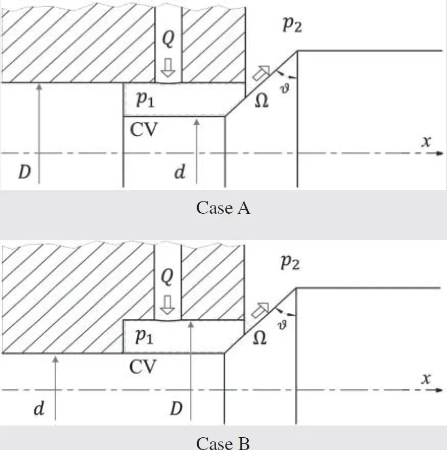
Determine an expression for the flow force acting on the valve poppet respectively for Case A and Case B. Assume that the valve poppet angle θ perfectly guides the flow at the valve exist section Ω.

Given:

Poppet valve geometry for two cases (figures above): flow rate Q ; exit area Ω; jet force angle θ ; and valve pressure drop Δ p = p 1− p 2

Find:

The expression and the direction of the flow force for Case A and Case B.

This example shows two possible cases of poppet valve design. With poppet valves, the flow exit area can be almost perfectly sealed when the valve is closed (poppet against the seat). This feature is very difficult to achieve with the spool valve geometries in Figure 3.17, due to the necessary clearance between the spool and the valve body.

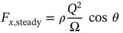
Flow force derivation – Case A

Equation (3.43)can be applied to the CV shown in the figure above, with the same assumptions illustrated in the previous paragraphs. This provides the expression of Eq. (3.48)for the flow force in steady state conditions:

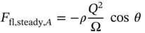
The flow force, in this case, tends to close the valve poppet.

Flow force derivation – Case B

Additionally, in this case, Eq. (3.43)can be applied to the CV shown in figure; however, it has to be noted that the Eq. (3.47)includes the overall contribution of the solid walls:

For this case, the pressure acting on CV at the left side (next to the entrance) is not acting on the sliding element, but on the valve body. It can be assumed that this pressure is equal to the entrance pressure p 1and uniformly distributed at the surface (i.e. small opening area Ω). Next, assuming that with the whole poppet downstream, the flow area Ω is at the pressure p 2:

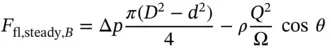
For typical valve geometries, it is easy to show that the first term is generally higher than the second one so that in this case the flow force tends to open the poppet.

This can be proven by writing the orifice equation that relates Q and Δ p :

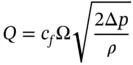
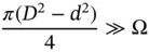
and considering that generally

1 3.1 The spool valve shown in the figure below has a maximum displacement of xv = 5 mm. The area ratio for the valve, in terms of opening area per unit travel of the spool, is w = 25 mm. Determine the maximum steady state flow force, considering the max working pressure conditions of 200 bar. Assume the jet angle to be 69° and a valve orifice coefficient of 0.7.

2 3.2 In an agricultural spraying system, the nozzles are supplied with water through 500 ft of aluminum (roughness, e = 5 10−6 ft) tubing from an engine driven pump. In its most efficient operating range, the pump output is 1500 gpm at a discharge pressure not exceeding 65 psi. For satisfactory operation, the sprinklers must operate at 30 psi or higher pressure.Minor losses and elevation changes may be neglected. Which is the smallest pipe size that can be used between: a 4‐in., a 5‐in., or a 6‐in. internal diameter pipe?

3 3.3 Water is pumped from a reservoir on a construction job site using the pipe system of the figure below. The flow rate must be 600 gm and water must leave the spay nozzle at 120 ft/s. The tubing piping system consists of a re‐entrant entrance, a regular 90°threaded elbow, two regular 45°threaded elbows, and a fully open gate valve (GV). The total length of the pipe is 700 ft, and the pipe has a diameter of 4 in.Calculate the total head loss of the system, including major and minor losses.Calculate the pump head required for the system.The following data can be used:Drawn tubing roughness: 5·10−6 ftRe‐entrant entrance loss coefficient: 0.890° elbow loss coefficient: 1.545° elbow loss coefficient: 0.4GV loss coefficient: 0.15