Andrea Vacca - Hydraulic Fluid Power
Здесь есть возможность читать онлайн «Andrea Vacca - Hydraulic Fluid Power» — ознакомительный отрывок электронной книги совершенно бесплатно, а после прочтения отрывка купить полную версию. В некоторых случаях можно слушать аудио, скачать через торрент в формате fb2 и присутствует краткое содержание. Жанр: unrecognised, на английском языке. Описание произведения, (предисловие) а так же отзывы посетителей доступны на портале библиотеки ЛибКат.

- Название:Hydraulic Fluid Power
- Автор:
- Жанр:
- Год:неизвестен
- ISBN:нет данных
- Рейтинг книги:3 / 5. Голосов: 1
-
Избранное:Добавить в избранное
- Отзывы:
-
Ваша оценка:
Hydraulic Fluid Power: краткое содержание, описание и аннотация
Предлагаем к чтению аннотацию, описание, краткое содержание или предисловие (зависит от того, что написал сам автор книги «Hydraulic Fluid Power»). Если вы не нашли необходимую информацию о книге — напишите в комментариях, мы постараемся отыскать её.
Readers of
will benefit from:
Approaching hydraulic fluid power concepts from an “outside-in” perspective, emphasizing a problem-solving orientation Abundant numerical examples and end-of-chapter problems designed to aid the reader in learning and retaining the material A balance between academic and practical content derived from the authors’ experience in both academia and industry Strong coverage of the fundamentals of hydraulic systems, including the equations and properties of hydraulic fluids
is perfect for undergraduate and graduate students of mechanical, agricultural, and aerospace engineering, as well as engineers designing hydraulic components, mobile machineries, or industrial systems.
Hydraulic Fluid Power — читать онлайн ознакомительный отрывок
Ниже представлен текст книги, разбитый по страницам. Система сохранения места последней прочитанной страницы, позволяет с удобством читать онлайн бесплатно книгу «Hydraulic Fluid Power», без необходимости каждый раз заново искать на чём Вы остановились. Поставьте закладку, и сможете в любой момент перейти на страницу, на которой закончили чтение.
Интервал:
Закладка:
The constant of proportionality in the quadratic equation between pressure can be referred to as turbulent hydraulic resistance, R turb. The resistance term originates from the electric analogy approach. The value of the resistance sets the link between the generalized flow variable (electric current, in the electric domain, and volume flow rate, in the hydraulic domain) and the generalized effort variable (voltage, in the electric domain and pressure, in the hydraulic domain) 2 :
(3.38) 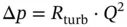
The hydraulic resistance R can be analytically derived from Eq. (3.29)(major losses) and Eq. (3.32)(minor losses), if the empirical friction factor or the loss coefficient is known. However, it is quite common for hydraulic components to find flow–pressure drop curves such as the one in Figure 3.14(valid for a check valve), from which the resistance coefficient can be easily derived.
At this point, the reader should notice one major difference between the hydraulic and electrical resistances. In fact, in the hydraulic domain, the law is quadratic, while in the electrical one (Ohm's law), it is linear. This is because of the turbulent flow condition. The hydraulic–electrical analogy is completely accurate only for laminar flow conditions:
(3.39) 
where R lamis the laminar hydraulic resistance. The subscript designation of the hydraulic resistance R is different between Eqs. (3.38)and (3.39)and refers to the type of flow inside the component. In hydraulic applications, laminar flow occurs only in particular cases, such as leakage flows inside the small gaps of pumps or spool valves.
The hydraulic resistanceexpresses the relation between flow rate Q and pressure drop Δ p across a hydraulic element. For laminar flow conditions, the hydraulic resistance R lamis a constant of proportionality between Q and Δ p . In the more common case of turbulent conditions, the hydraulic resistance is a coefficient between Q 2and Δ p .
For simplified studies, or when linear relations are more convenient for applying control laws, it is possible to assume a linear relation between flow rate and pressure also for turbulent flow. This approximation is not recommended for general analysis, but it can be accurate enough to describe relative variations of pressure and flows in a small interval, as it is illustrated in Figure 3.15.
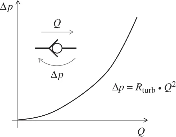
Figure 3.14 Resistance across a hydraulic check valve.
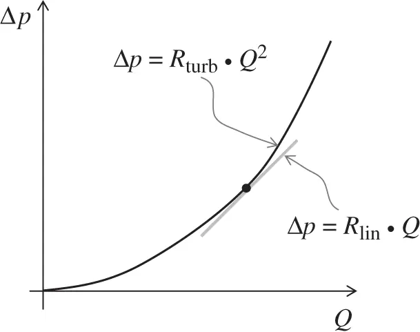
Figure 3.15 Linear approximation for the hydraulic resistance in turbulent flow conditions.
The linear hydraulic resistance ( R lin) can be calculated as
(3.40) 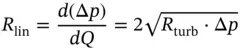
3.7 Stationary Modeling of Flow Networks
The following chapters of the book focus on the analysis of hydraulic systems operating in steady‐state conditions. Hence, after the presentation of the basic equations for hydraulic resistance and conservation of mass, it is now appropriate to provide the reader with the general approach that can be used to model a flow network.
A flow network can be defined as any collection of elements (valves, cylinders) and sources (pumps). The network interconnections are the fluid conveyance elements.
According to the approach also presented by Merritt [32], the flow and the pressure distribution within a network must satisfy three constraints:
1 Flow–pressure relationshipEvery element of the circuit is characterized by a flow–pressure relationship. The simplest example is the case of the hydraulic resistance that can be used to describe pipes, fittings, and certain hydraulic valves, previously shown in Eqs. (3.38)and (3.39). The next chapters will present also relations for other elements, such as pumps, motors, and linear actuators.
2 Flow lawThe flow law applies at any junction of pipes, and it was already presented as a direct consequence of the conservation of mass principle: (3.41)Equation (3.41) can be seen as the equivalent of the Kirchhoff's current law in the electric domain. Essentially, this equation states that the sum of the flow rates entering a junction has to be equal to the sum of the flow rates exiting it ( Figure 3.16a).
3 Pressure lawThe pressure law can be seen as the equivalent of the Kirchhoff's voltage law in the electric domain. It states that the overall pressure drop around any closed circuit has to be null:(3.42)
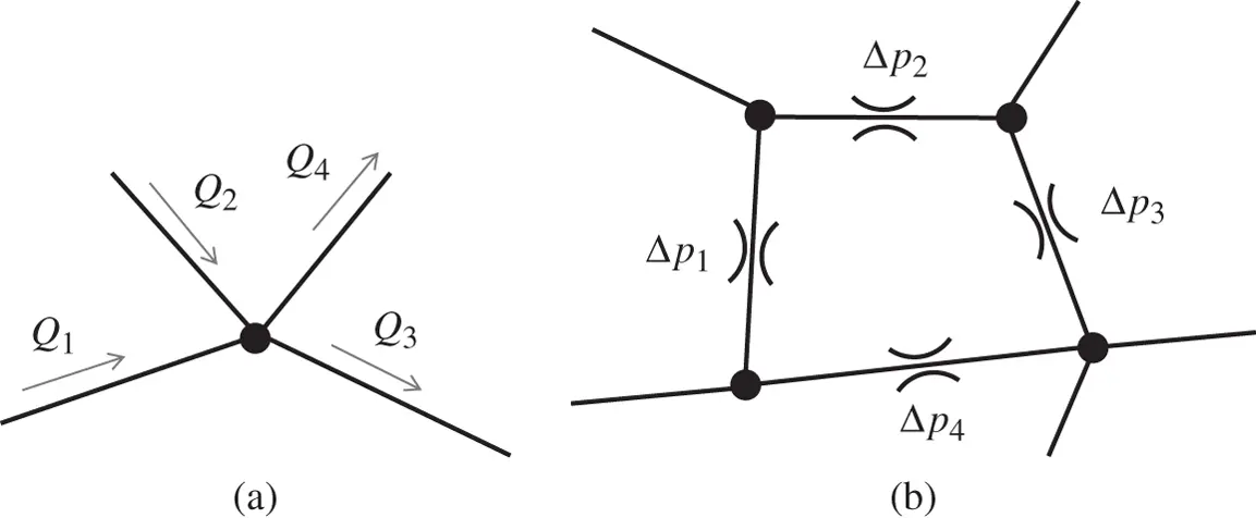
Figure 3.16 Graphical representation of flow law (a) and pressure law (b).
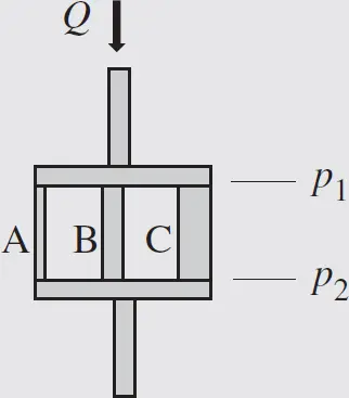
Example 3.1 Series and parallel hydraulic connections
The pressure drop–flow rate relation for three different pipes is known to be linear, as shown in the figure below. Find the pressure drop–flow rate relation for different configurations of the three pipes: (a) series; (b) parallel; and (c) series–parallel.
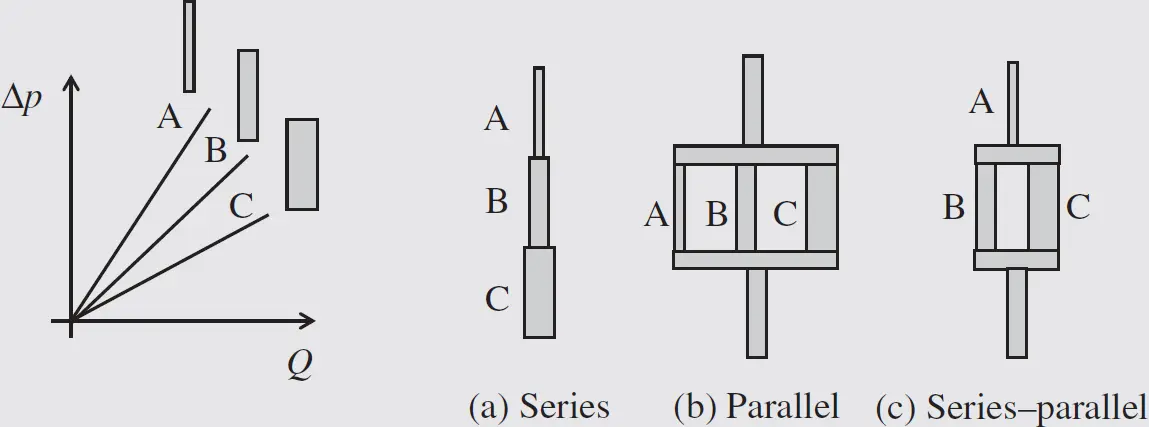
Given:
The linear characteristic of three pipe sections:
Δ p A= R A· Q A; Δ p B= R B· Q B; Δ p C= R C· Q C
Find:
The equivalent hydraulic resistance for the three cases:
Δ p series= R series· Q ; Δ p parallel= R parallel· Q ; Δ p series/parallel= R C· Q
Solution:
Case (a) series
This case can be solved by considering the quantities shown in the figure below:
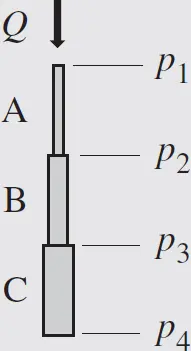

Therefore,

which means
Case (b) parallel
The approach is similar to case (a). With reference to the figure below,

Considering the flow law,
Читать дальшеИнтервал:
Закладка:
Похожие книги на «Hydraulic Fluid Power»
Представляем Вашему вниманию похожие книги на «Hydraulic Fluid Power» списком для выбора. Мы отобрали схожую по названию и смыслу литературу в надежде предоставить читателям больше вариантов отыскать новые, интересные, ещё непрочитанные произведения.


Обсуждение, отзывы о книге «Hydraulic Fluid Power» и просто собственные мнения читателей. Оставьте ваши комментарии, напишите, что Вы думаете о произведении, его смысле или главных героях. Укажите что конкретно понравилось, а что нет, и почему Вы так считаете.