Andrea Vacca - Hydraulic Fluid Power

For the regions of fully developed flow, it is possible to analytically demonstrate that for laminar flow conditions:

(3.28)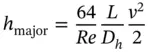

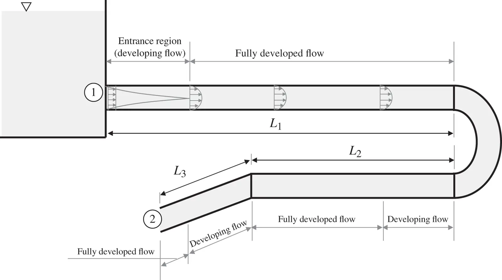
Figure 3.11 Example of analysis of major and minor losses in a pipe flow.

The velocity value v represents the average velocity over the section. From considerations based on dimensional analysis, it is possible to derive the Darcy‐Weisbach equation, which has validity for both laminar and turbulent flow conditions:

(3.29)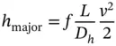

where the friction factor f is a function of the Reynolds number and the relative roughness of the pipe:

(3.30)

Figure 3.12shows the results from the pioneering work performed by Moody [15] on the determination of the friction factor. The Moody's diagram is nowadays the most used chart for determining the major head losses in pipe flows. Analytical expressions for f can also be found in basic fluid mechanics textbooks. A widely adopted one is the Colebrook's formula:

(3.31)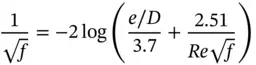

From Eq. (3.28), it is possible to conclude that the loss term h majorin laminar conditions is proportional to the average fluid velocity ( v ) because of the presence of the Reynolds number, Re , at the denominator of the expression. However, under conditions of complete turbulence, where the friction factor f is constant, the loss term follows a quadratic relation with v .

The major loss term h majoris proportional to the average fluid velocity, v , in laminar conditions, and to v 2in complete turbulent conditions.

Minor losses are primarily caused by flow separation effects. Figure 3.13illustrates the case of the flow separation in proximity of a pipe entrance from a reservoir: the streamlines qualitatively illustrated the mixing areas of the separated zones, where energy is dissipated.

Flow separation effects such as the case in Figure 3.13occur at every geometrical discontinuity of the pipe flow system. The energy losses in these cases are described by two alternative formulas:

(3.32)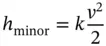

or

(3.33)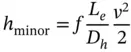

As in the case of major losses, minor losses are quantified with respect to the kinetic term v 2/2, by means of empirical relations based on experimental data. For many cases, particularly for entrances, exits, or sudden contractions or expansions, it is common to find in the literature the k coefficients. In the case of an exit to a tank, it is intuitive to consider that all the kinetic energy of the fluid inside the pipe will be dissipated; therefore, k exit= 1. For other discontinuities, typically k < 1.

For other discontinuities, such as elbow or bends, it is more common to evaluate the friction coefficient f relative to the diameter representative of the discontinuity (i.e. the diameter of the curved pipe, for the case of an elbow) and use an empirical value of equivalent length L e, which corresponds to the length of a straight pipe that would provide the same head loss.

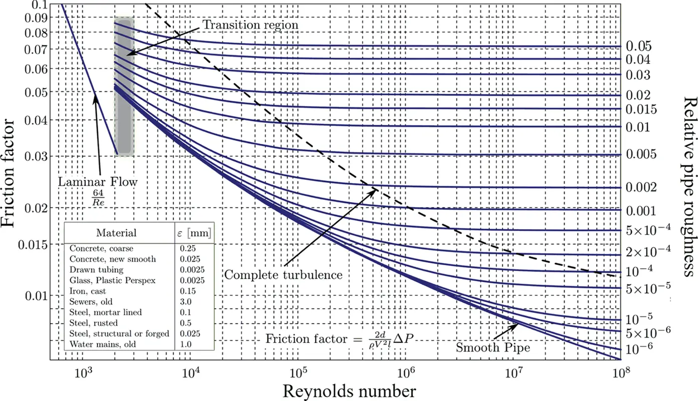
Figure 3.12 Moody's diagram for the calculation of the friction factor.

Source: Moody's diagram, Darcy–Weisbach friction factor, wikipedia. Licensed under CC BY‐SA 4.0.

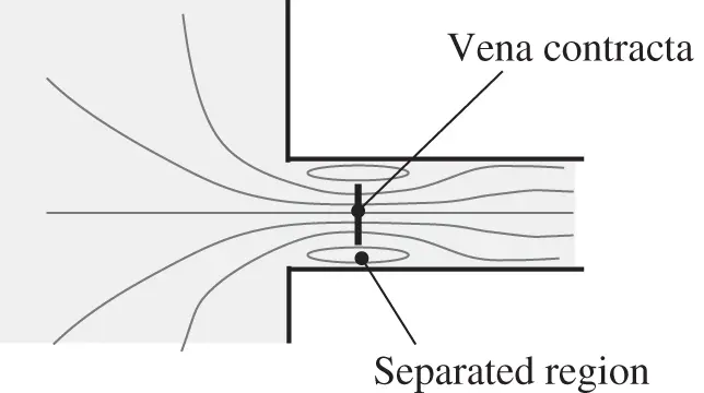
Figure 3.13 Example of separation region at a flow entrance.

A fluid power engineer must be ready to use both the formulas (3.32)and (3.33), depending on the data source that is available. For basic geometries, empirical data for minor losses can be found in the book of Idelchik [31].

It is important to point out that, in general, the minor losses include also the frictional effects of the developing flow region that follows the initial flow separation. This allows for a straightforward identification of the lengths to be used in the evaluation of the major loss terms. For example, with reference to the previous Figure 3.11, the entrance loss considers the additional losses associated to the entrance region in such a way that the evaluation of the major losses of the first straight section of the pipe is performed with the geometrical length L 1. Similarly, the lengths L 2and L 3will be used in Eq. (3.29)for the other major losses present between the reference sections.

In most cases, the minor loss term h minoris proportional to the term v 2.

The generalized Bernoulli's law ( Eq. (3.25)) can be written differently to break down the energy losses into three different contributions:

(3.34)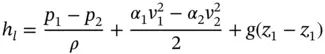

Equation (3.34)highlights the pressure, kinetics, and elevation terms contributing to h loss. In hydraulic systems, it is very common to have the pressure differential term dominating the other two, which can easily be ignored. For this reason, it can often be assumed that

(3.35)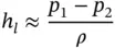

In hydraulic systems, the head loss term h l(= h major+ h minor) relates to a pressure loss.

Equations (3.25), (3.29)(major losses), and (3.32)(minor losses) highlight how the pressure drop due to frictional losses across a hydraulic element or a section of a pipe is proportional to v 2, for turbulent conditions:

(3.36)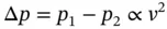

Common components of a hydraulic system such as valves and hydraulic fittings are mostly characterized by turbulent flow conditions. This is common for all sources of minor losses. Considering the relation between average velocity and volumetric flow rate ( Eq. (3.10)), Eq. (3.36)can be written as follows:

(3.37)