Sergey N. Makarov - Antenna and EM Modeling with MATLAB Antenna Toolbox

%% Setup analysis parameters f = linspace(200e6, 1200e6, 1000); % Frequency in Hz lA = 0.15; % Dipole total length, m a = 0.002; % Dipole radius, m %% Antenna toolbox model and analysis w = cylinder2strip(a); % Eq. strip width model d = dipole('Length',lA,'Width',w); % Strip dipole model figure; show(d) % Visualize geometry Z = impedance(d, f); % Full-wave MoM solution R = real(Z); % Resistance X = imag(Z); % Reactance

Emphasize that the numerical solution uses an infinitesimally thin feed gap for the dipole antenna. An extension to a gap of finite thickness is possible.

We have already mentioned that, if a strip or blade dipole of width t is considered, then a twice as narrow cylindrical dipole provides the same equivalent capacitance of a dipole wing per unit length [3]. For example, the blade dipole of 8 mm in width and the cylindrical dipole of 4 mm in diameter should perform quite similarly.

The results from our numerical experiment suggest that the existing theory model is a good approximation for dipoles around the first resonance. Eq. (1.14)indeed quickly loses its validity above the first antenna resonance. The numerical model is also not perfect, but it is perhaps more reliable. We emphasize that the dipole theory model is still extremely useful in the estimation of the antenna path loss where its accuracy is quite sufficient; this question will be considered in the following text.

1 1. D. R. Jackson, “Microstrip Antennas,” In Antenna Engineering Handbook, J. L. Volakis, Ed., McGraw Hill, New York, 2018, fifth edition.

2 2. C. ‐T. Tai and S. A. Long, “Dipoles and Monopoles,” In Antenna Engineering Handbook, J. L. Volakis, Ed., McGraw Hill, New York, 2007, fourth edition.

3 3. C. A. Balanis, Antenna Theory: Analysis and Design, Wiley, New York, 2016, fourth edition.

1 1. A small AM radio antenna operating at 1 MHz uses a thin copper wire with the diameter D of 0.2 mm and with the total wire length of 3 m.Calculate parasitic antenna's resistance (loss resistance) RL.What is the antenna efficiency percentage if the radiation resistance is 1 Ω?

2 2. In Example 1.4, we replace the 62 mil FR4 substrate by a Rogers substrate material RO4003 with the same thickness and with εr=3.55 and tan δ=0.0027. Is the efficiency of the patch antenna improved? What is the new efficiency value?

3 3. The generator's voltage source creates a sine wave with the amplitude of 10 V. The generator resistance is Rg = 50 Ω. The antenna impedance at a frequency of interest measuresΖa = 50 Ω + j0 Ω;Ζa = 75 Ω + j0 Ω;Ζa = 25 Ω + j0 Ω;Ζa = 50 Ω + j50 Ω;Ζa = 50 Ω − j50 Ω;Ζa = 50 Ω + j100 Ω.In every case, determineAverage power delivered to the antenna (show units).Average power radiated by the antenna assuming loss resistance of 10 Ω in every case.

4 4. The following antenna impedances are tested:Ζa = 75 Ω + j10 Ω;Ζa = 25 Ω + j0 Ω;Ζa = 50 Ω + j25 Ω.Which antenna is best matched to the generator resistance of 50 Ω (is characterized by the highest accepted power)?

5 5*. Approximately determine the resonant frequency of a strip dipole with the total length of 100 mm and the width of 2 mm. Prove your answer using MATLAB Antenna Toolbox and find the error. Present the text of the corresponding MATLAB script.

6 6*. Generate Figure 1.6in MATLAB. Present the text of the corresponding MATLAB script.

7 7*.Draw the equivalent circuit for a generic transmitting antenna in frequency domain including the generator and the antenna. Label all circuit parameters.How do we define the “resonant” antenna condition?Create a strip dipole in MATLAB Antenna Toolbox with the length of 30 cm and the width of 2 mm. Use the impedance function over the frequency band 300–600 MHz and identify the frequency at which the antenna is resonant.What is the antenna radiation resistance at the resonance (assuming the lossless antenna)?Attach your MATLAB script to the homework report.

8 8*.Does the resonant frequency of a strip dipole increase or decrease with increasing its width? Prove your answer using MATLAB Antenna Toolbox.Does the resonant frequency of a cylindrical dipole increase or decrease with increasing its radius? Justify your answer.

9 9*. Use the dipole modeled in problem 7 C and analyze the impedance over the frequency band 300 MHz–1.5 GHz. Find all the series resonances in the impedance plot and annotate them. Report your results on the relationship between the resonant frequencies relative to the first resonance.

10 10*. In MATLAB Antenna Toolbox, the amplitude of the port excitation voltage of the strip dipole antenna changes from 1 to 2 V. How will the antenna impedance change?

1 1.8 Antenna Reflection Coefficient for a Lumped Circuit

2 1.9 Antenna Reflection Coefficient with a Feeding Transmission Line

3 1.10 Antenna Impedance Transformation. Antenna Match Via Transmission Line

4 1.11 Reflection Coefficient Expressed in Decibels and Antenna Bandwidth

5 1.12 VSWR of the Antenna

6 References

7 Problems

If an antenna is connected to the generator via a short cable with the length being small compared to the wavelength, the lumped circuit in Figure 1.3is entirely sufficient for antenna modeling. In practice, however, the antenna is usually connected via a longer cable. The cable connections are also common in antenna arrays ; they are used to construct the beamforming networks .

Voltage and currents on long cables (transmission lines) are in fact electromagnetic waves, which may propagate back and forth between the antenna and the generator. A method of scattering parameters or S‐parameters is useful in this case. S‐parameters describe the complete behavior of a high‐frequency distributed linear circuit . The term “scattering parameters” comes from the “Scattering Matrix” described in a 1965 IEEE article by K. Kurokawa entitled “Power Waves and the Scattering Matrix.” Today, S ‐parameter results are displayed on the vector network analyzer display screen with the simple push of the button.

We will consider the lumped circuit in Figure 1.3first, with a real generator impedance, R g, and an arbitrary antenna impedance, Z a. The ratio of the available power delivered to the antenna (1.13c)to the maximum available power (1.13d)for the ideal match gives us an important parameter, the normalized power delivered to the antenna :

(1.16)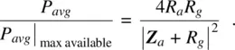

This result is nicely expressed in terms of the complex reflection coefficient (or voltage reflection coefficient ), Γ, which is given by a combination of generator and antenna impedances [1]:

(1.17)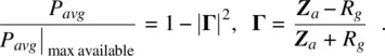

The corresponding proof task is cast as a homework problem at the end of this chapter. Emphasize that, if the antenna is connected to a microstrip transmission line or a cable, then R gis replaced by the characteristic impedance of the transmission line, Z 0, i.e. R g→ Z 0.