Sergey N. Makarov - Antenna and EM Modeling with MATLAB Antenna Toolbox
Здесь есть возможность читать онлайн «Sergey N. Makarov - Antenna and EM Modeling with MATLAB Antenna Toolbox» — ознакомительный отрывок электронной книги совершенно бесплатно, а после прочтения отрывка купить полную версию. В некоторых случаях можно слушать аудио, скачать через торрент в формате fb2 и присутствует краткое содержание. Жанр: unrecognised, на английском языке. Описание произведения, (предисловие) а так же отзывы посетителей доступны на портале библиотеки ЛибКат.
- Название:Antenna and EM Modeling with MATLAB Antenna Toolbox
- Автор:
- Жанр:
- Год:неизвестен
- ISBN:нет данных
- Рейтинг книги:4 / 5. Голосов: 1
-
Избранное:Добавить в избранное
- Отзывы:
-
Ваша оценка:
Antenna and EM Modeling with MATLAB Antenna Toolbox: краткое содержание, описание и аннотация
Предлагаем к чтению аннотацию, описание, краткое содержание или предисловие (зависит от того, что написал сам автор книги «Antenna and EM Modeling with MATLAB Antenna Toolbox»). Если вы не нашли необходимую информацию о книге — напишите в комментариях, мы постараемся отыскать её.
Antenna and EM Modeling with MATLAB Antenna Toolbox — читать онлайн ознакомительный отрывок
Ниже представлен текст книги, разбитый по страницам. Система сохранения места последней прочитанной страницы, позволяет с удобством читать онлайн бесплатно книгу «Antenna and EM Modeling with MATLAB Antenna Toolbox», без необходимости каждый раз заново искать на чём Вы остановились. Поставьте закладку, и сможете в любой момент перейти на страницу, на которой закончили чтение.
Интервал:
Закладка:
In the general case of generator(s) and load(s) connected by cables/transmission lines, whose length is comparable to the wavelength, the reflection coefficient is formed by two voltage or power waves [1]. The incident wave V +propagates along a cable (the transmission line) from the generator depicted in Figure 1.3‐left toward the antenna load. The reflected wave V −propagates along the same cable but in the opposite direction, i.e. from the antenna to the generator. The complete voltage solution is the sum of both. The complex reflection coefficient of the antenna with a cable is defined as the ratio of two complex voltage values at the generator,
(1.18) 
If there is no reflected wave, the reflection coefficient is exactly zero and there is an ideal match in Eq. (1.17). The transmitted wave is completely acquired by the antenna and is then radiated into the surrounding space.
The meaning of transmitted and reflected power waves is extremely useful in measurements (the vector network analyzer) and specifically for modeling networks with transmission lines (cables) of a significant length where the electromagnetic waves can propagate in a nontrivial way (change the phase or decay).
The size of the lumped circuit in Figure 1.3was assumed to be negligibly small compared to the wavelength. In this case, both contributions  and
and  may be deduced from the standard circuit analysis of lumped circuits (we use index 0 to distinguish this particular case). In that case, the meaning of the reflection coefficient is reduced to the standard circuit analysis; it simply reflects generator resistance and antenna impedance mismatch studied previously.
Example 1.7
Find  and
and  for the lumped TX circuit shown in Figure 1.3‐right.
Solution:The “incident voltage wave” is the antenna voltage for the ideal match,
(1.19) 
The “reflected voltage wave” is simply the actual antenna voltage minus the voltage for the ideal match, that is
(1.20) 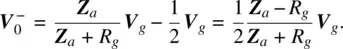
Their ratio is given by
(1.21) 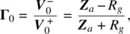
which is exactly Eq. (1.17). The reference plane (at either generator or the antenna load) does not matter for the lumped circuit.
1.9 ANTENNA REFLECTION COEFFICIENT WITH A FEEDING TRANSMISSION LINE
Now, consider a generator connected to the antenna through a lossless transmission line (a coaxial cable, a printed microstrip, or a waveguide). The familiar lumped circuit in Figure 1.7a (and Figure 1.3) is transformed as shown in Figure 1.7b. In many practical situations, the transmission line is precisely matched to the generator; its characteristic impedance Z 0is chosen to be equal to the generator resistance, that is
(1.22) 
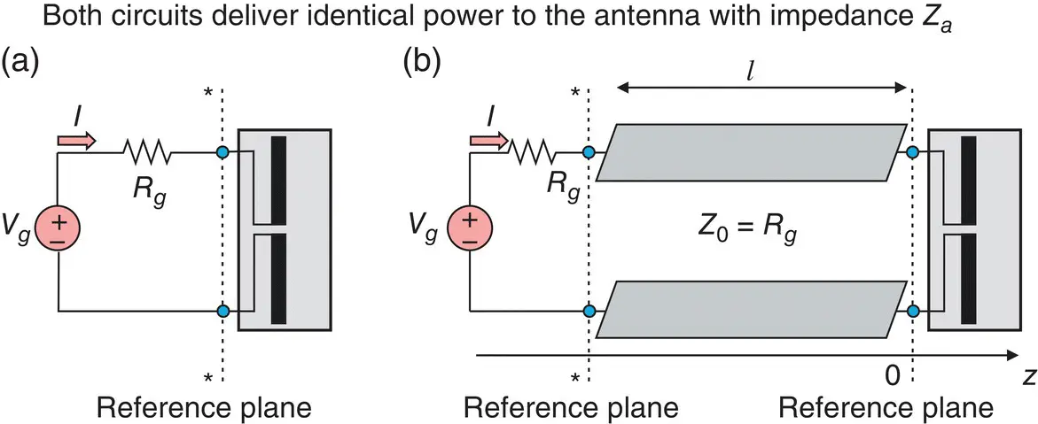
Figure 1.7 Equivalence of the TX circuits with and without the transmission line from the viewpoint of the power delivered to the antenna.
Our goal is to find the reflection coefficient of the combined system consisting of the antenna and the transmission line of length l in Figure 1.7b. The z ‐axis will be directed from the source to the antenna along the transmission line. To be consistent with the lumped‐circuit approach from Example 1.7, we set the origin of the z ‐axis ( z = 0) in the antenna reference plane in Figure 1.7b. Then, both the incident (traveling to the right) and the reflected (traveling to the left) waves in Figure 1.7b will have the following phasor form (time dependence is exp ( jωt )):
(1.23) 
according to the familiar one‐dimensional plane wave theory. Here, k is the real wavenumber of the lossless transmission line. It is equal to the angular frequency divided by the phase velocity (propagation speed), c , of the line. Voltage wave V +propagates from left to right and corresponds to cos ( ωt − kz ) in time domain while voltage wave V −propagates from right to left and corresponds to cos ( ωt + kz ). Note that k = β in Pozar's book [1].
According to Eq. (1.18)and (1.23), the reflection coefficient of the antenna with the transmission line in reference plane * in Figure 1.7b, i.e. at the generator where z = − l , has the form:
(1.24) 
where Γ 0is given by Eq. (1.21)with R g= Z 0. When transmission line length tends to zero, Eq. (1.24)is indeed reduced to Eq. (1.21). Eq. (1.24)is a simple yet powerful result; it will predict the average power delivered to the antenna with a cable or another transmission line.
Example 1.8shows that the addition of the lossless transmission line perfectly matched at the generator does that change average power delivered to the antenna, irrespective of the value of its input impedance.
Example 1.8
Show that the addition of a lossless transmission line of any length, which is still perfectly matched at the generator, does not change average power delivered to the antenna of any input impedance. Only a phase of the reflection coefficient at the generator changes.
Solution:The solution is based on Eq. (1.24), which yields
(1.25) 
Therefore, according to Eq. (1.17),
(1.26) 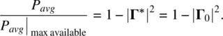
Интервал:
Закладка:
Похожие книги на «Antenna and EM Modeling with MATLAB Antenna Toolbox»
Представляем Вашему вниманию похожие книги на «Antenna and EM Modeling with MATLAB Antenna Toolbox» списком для выбора. Мы отобрали схожую по названию и смыслу литературу в надежде предоставить читателям больше вариантов отыскать новые, интересные, ещё непрочитанные произведения.


Обсуждение, отзывы о книге «Antenna and EM Modeling with MATLAB Antenna Toolbox» и просто собственные мнения читателей. Оставьте ваши комментарии, напишите, что Вы думаете о произведении, его смысле или главных героях. Укажите что конкретно понравилось, а что нет, и почему Вы так считаете.