Sergey N. Makarov - Antenna and EM Modeling with MATLAB Antenna Toolbox

%% Setup analysis parameters f = linspace(200e6, 1200e6, 1000); % Frequency, Hz lA = 0.15; % Dipole total length, m a = 0.002; % Dipole radius, m %% Antenna toolbox model and analysis w = cylinder2strip(a); % Eq. strip width model d = dipole('Length',lA,'Width',w); % Strip dipole model figure; show(d) % Visualize geometry S11 = rfparam(sparameters(d,f,Rg),1,1); % Calculate s-parameters S11dB = 20*log10(abs(S11));

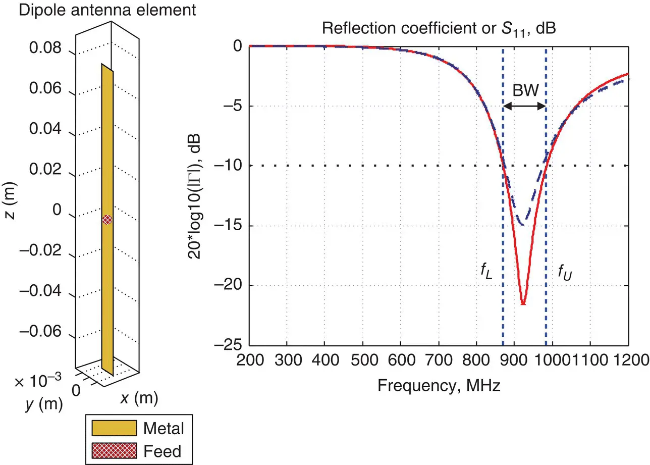
Figure 1.8Magnitude of the reflection coefficient in dB for the dipole antenna and the antenna impedance bandwidth. Numerical solution is shown by a dashed curve.

In Figure 1.8, the antenna impedance bandwidth follows Eq. (1.32)or (1.34)with the minus 10 dB threshold. The threshold is shown by two dashed lines in Figure 1.8. The dipole antenna has the impedance bandwidth from the lower frequency of the band , f L= 870.7 MHz, to the upper frequency of the band , f U= 985.8 MHz (analytical solution is considered as an example). The center frequency of the band is given by

(1.35)

The antenna impedance bandwidth BW (or fractional bandwidth) is determined in the form

(1.36)

which is a very typical value for a wire dipole or a thin‐blade dipole. Generally, we always want to increase the antenna bandwidth for a better throughput.

Eq. (1.36)determines the bandwidth when it does not exceed 100%. For broadband antennas, the bandwidth is alternatively determined by the ratio of the upper‐to‐lower frequencies,

(1.37)

Both definitions may overlap. For example, if f U= 1GHz, f L= 500MHz, the antenna bandwidth according to Eq. (1.36)is 67% whereas the antenna bandwidth according to Eq. (1.37)is 2 : 1.

Along with the reflection coefficient Γor S 11, another measurable quantity of significant interest is the voltage standing‐wave ratio or VSWR. On a transmission line connected to non‐matched antenna, both waves – incident and reflected V +and V −, respectively – form a prominent standing wave. At every point in space, this standing wave has a certain amplitude as a sinusoidal function of time. The VSWR is given by the ratio of maximum and minimum standing wave amplitudes on the line. It may be shown that [1–3]

(1.38a)

For the matched antenna, the VSWR is exactly one; for a non‐matched antenna, it is always greater than one, and may even approach infinity for a short‐ or open‐circuited antenna.

The VSWR may be used instead of the reflection coefficient to determine and plot the impedance bandwidth. In this case, the criterion of

(1.38b)

corresponds to

(1.38c)

with a sufficient degree of accuracy.

Plot the reflection coefficient in dB and VSWR for the dipole with l A= 15 cm, a = 2 mm over the band 200–1200 MHz using Eq. (1.14)and MATLAB, and determine the antenna impedance bandwidth.

Solution:We repeat the task of Example 1.5, but instead of the impedance plot, the reflection coefficient and the VSWR will be evaluated and plotted. Extra lines of the MATLAB code may be added such as

c = figure; Rg = 50; RC =(Za-Rg)./(Za+Rg); temp = abs(RC); VSWR = (1 + temp)./(1 - temp); semilogy(f/1e6, VSWR, 'b', 'LineWidth', 2); grid on; xlabel ('frequency, MHz'); ylabel ('VSWR, a.u.'); title('VSWR');

The result is shown in Figure 1.9. The same antenna impedance bandwidth is marked on every plot – for the reflection coefficient and for the VSWR, respectively. In fact, the VSWR ≤ 2 bandwidth on the right plot is slightly greater than the | Γ| dB≤ − 10 dB bandwidth since, strictly speaking, the condition VSWR = 2 corresponds to | Γ| dB= − 9.5 dB. This difference is usually ignored.

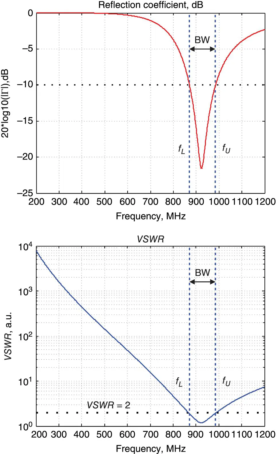
Figure 1.9 Reflection coefficient in dB (left) versus VSWR (right) for the same dipole antenna.

1 1. D. M. Pozar, Microwave Engineering, Wiley, New York, 2011, fourth edition.

2 2. T. A. Milligan, Modern Antenna Design, Wiley, New York, 2005, second edition, pp. 17–18.

3 3. C. A. Balanis, Antenna Theory: Analysis and Design, Wiley, New York, 2016, fourth edition.

1 1. An antenna withΖa = 100 ΩΖa = 100 Ω − j100 ΩΖa = 100 Ω + j100 Ωis directly connected to a generator with Rg = 50 Ω. Determine the reflection coefficient Γ of the antenna, its magnitude, and normalized power delivered to the antenna in every case.

2 2. Repeat Problem 1 ifa quarter wave transmission line with Z0 = 70.7 Ω is added to the antenna;a full wave transmission line with Z0 = 70.7 Ω is added to the antenna.

3 3. If an antenna is either an open or short circuit, what is its reflection coefficient, Γ? Hint: The problem may be solved using the currents associated with the reflected and forward waves in Eq. (1.18), but introducing a minus sign to account for the opposite orientations of the two currents: .

4 4. Repeat Problem 3 ifa quarter wave transmission line with Z0 = Rg is added to the antenna;a full wave transmission line with Z0 = Rg is added to the antenna.

5 5. The exact values of the antenna reflection coefficient Γ (computed vs. characteristic impedance of a 50 Ω transmission line) are0.1;0.316;−0.5.Determine the reflection coefficient values in dB.Determine antenna impedance.

6 6. Calculate and plot to scale the phase of the reflection coefficient in Example 1.10.

7 7. In Example 1.10, a coaxial transmission cable RG‐58 with Ζ0 = Rg = 50 Ω and with the length of 1 m is added to the antenna. How does the plot in Figure 1.8change?

8 8. The lower frequency of an antenna band is 2.5 GHz; the upper frequency of the band is 6 GHz. Determine the band center frequency and the antenna impedance bandwidth.

9 9. In Example 1.10, we use a generator with Rg = 100 Ω. How does the antenna impedance bandwidth will change?

10 10*. A thick cylindrical tubular dipole has lA = 15 cm, a = 5 mm. Using MATLAB Antenna Toolbox, determine the center frequency of the band and the impedance bandwidth percentage. How do those values relate to the values found in Example 1.10?