Sergey N. Makarov - Antenna and EM Modeling with MATLAB Antenna Toolbox

In Eq. (1.14), l Ais the total dipole length, a is the dipole radius, z = kl A/2, and is the wavenumber with c 0being the speed of light in vacuum.

If a strip or blade dipole of width t is considered, then a eq= t /4 [3] (providing the same equivalent capacitance of a dipole wing per unit length). We note here that a is the radius of a cylindrical dipole, while a eqis the equivalent radius of a wire approximation to the strip dipole. Eq. (1.14)holds for relatively short nonresonant dipoles and for half‐wave dipoles, i.e. in the frequency domain approximately given by

(1.15)

where f res≡ c 0/(2 l A) is the resonant frequency of an idealized dipole having exactly a half‐wave resonance ( c 0is again the speed of light) and f Cis the center frequency of the band. This means that the ideal dipole resonates when its length is the half wavelength. When a monopole over an infinite ground plane is studied, the impedance in Eq. (1.14)halves.

Plot to scale the input impedance for a dipole antenna with l A= 15 cm, a = 2 mm and over the band 200–1200 MHz using Eq. (1.14)and MATLAB.

Solution:First, we find the resonant frequency of an idealized dipole, which is f res= c 0/(2 l A) = 3 × 10 8/0.3 = 1 GHz. A simple MATLAB script given below uses Eq. (1.14)and outputs the plot shown in Figure 1.5for the dipole impedance. One can see that the true resonance occurs at a bit lower frequency of 928 MHz; the resonant radiation resistance appears to be 60 Ω. According to Figure 1.2, this is still a very good match, which is close to the maximum radiated antenna power.

f = linspace(200e6, 1200e6, 1000);% Frequency, Hz lA = 0.15; % Dipole total length, m a = 0.002; % Dipole radius, m Za = dipoleAnalytical(f, lA, a); % Find resonant frequency Ra = real(Za); Xa = imag(Za); % Find resistance and reactance [dummy, index] = min(abs(Xa)); % Find resonant frequency fresMHz = f(index)/1e6 hold on; grid on; plot(f/1e6, Ra, 'b', 'LineWidth', 2); plot(f/1e6, Xa, 'r', 'LineWidth', 2); xlabel ('frequency, MHz'); ylabel ('Impedance, \Omega'); axis([min(f)/1e6 max(f)/1e6 -200 200]); title('Dipole resistance(blue) and reactance(red), \Omega'); line([fresMHz fresMHz],[-200 200]);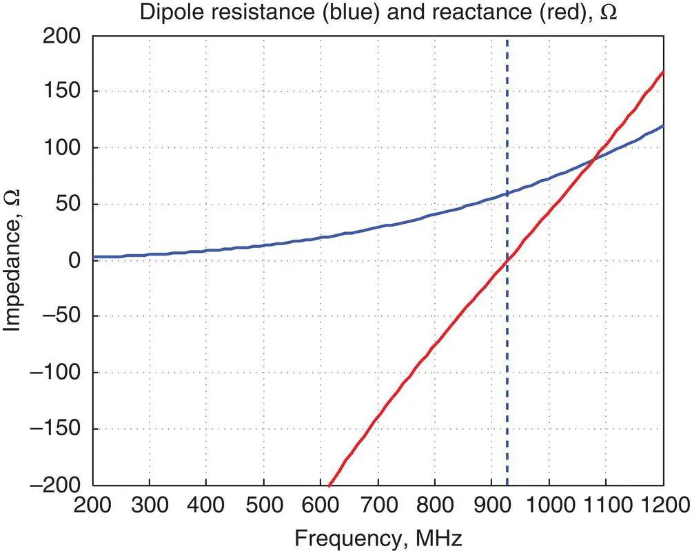

Figure 1.5 Dipole antenna impedance in the vicinity of its first (series) resonance. The dashed line shows the resonant frequency.

The MATLAB script above uses function dipoleAnalyticalthat corresponds to Eq. (1.14):

function [Za] = dipoleAnalytical(f, lA, a); % EM data epsilon = 8.85418782e-012; % Vacuum, F/m mu = 1.25663706e-006; % Vacuum, H/m c = 1/sqrt(epsilon*mu); % Vacuum, m/s eta = sqrt(mu/epsilon); % Vacuum, Ohm l = lA/2; % Dipole half length k = 2*pi*f/c; % Wavenumber z = k*l; % Electrical length corresponding to l R = -0.4787 + 7.3246*z + 0.3963*z.^2 + 15.6131*z.^3; X = -0.4456 + 17.0082*z - 8.6793*z.^2 + 9.6031*z.^3; Za = R - j*( 120*(log(l/a)-1)*cot(z)-X ); % Antenna impedance end

We will show later in the text that all metal antennas could be scaled in size so that a dipole with the size twice as small as the original one has the resonant frequency that is two times larger than the original resonant frequency. Similarly, a dipole with the size twice as large as the original one has the resonant frequency that is two times less. In other words, small antennas have high resonant frequencies and vice versa.

The scaling property of the antenna implies measuring its length l Ain terms of a dimensionless quantity called electrical length . The electrical length is simply the product of l Aand the wavenumber k = 2 π / λ . The electrical length of the antenna does not depend on its operation frequency. A dipole antenna resonating at 100 MHz or at 5 GHz has the same electrical length.

The dipole antenna discussed thus far is a classic example of a narrow‐band antenna that has its first resonance as a series resonance. In general, a resonance is characterized by a zero reactance, X a= 0. However, the resistance value can vary dramatically depending on the type of resonance, i.e. series or parallel. Parallel resonances typically achieve large resistances. In the case of the dipole, the series resonances occur at odd multiples of f res. In general, the dipole is not used at higher multiples of the fundamental resonance. The half‐wavelength current distribution is no longer valid at these frequencies and therefore the radiation pattern of the antenna is also distorted.

Although impedances of many basic antenna types and geometries (dipoles, loops, patch antennas) are well documented (in particular, in Antenna Engineering Handbook , John L. Volakis, Ed., McGraw Hill, 2018, fifth edition), any particular antenna design heavily relies upon numerical electromagnetic modeling.

Let us compare the theoretical model for the dipole antenna impedance with a numerical model. The theoretical model is based on a cylindrical dipole (1.14). The modeling software used in this text is the Method of Moments software of the MATLAB ®Antenna Toolbox ™. This software has a library of antenna models that are parameterized to enable easy geometry setup and analysis. One such model is the dipole.

This model of the dipole in MATLAB will use the strip or blade approximation of the cylindrical dipole as discussed in [3]. We consider the same dipole as in Example 1.5, with the total length of 15 cm, and with the radius of 2 mm, and then compare its theoretical impedance model given by Eq. (1.14)with numerical simulations, in the band from 200 to 1200 MHz. As discussed above, the equivalent radius of the strip dipole of width t is a eq= t /4.

Using MATLAB Antenna Toolbox, compare theory and numerical simulations for the strip dipole antenna with l A= 15 cm, t = 8 mm over the band 200–1200 MHz. The theory model uses Eq. (1.14).

Solution:A simple MATLAB script given below initializes the dipole antenna, plots the antenna geometry, and computes the dipole input impedance over the frequency band of interest at the default computational mesh resolution. Figure 1.6shows the resulting dipole geometry and the impedance comparison. The agreement between two solutions is good in the middle of the band, but it becomes worse at higher frequencies and at very low frequencies. There, the numerical solution generally becomes more accurate.

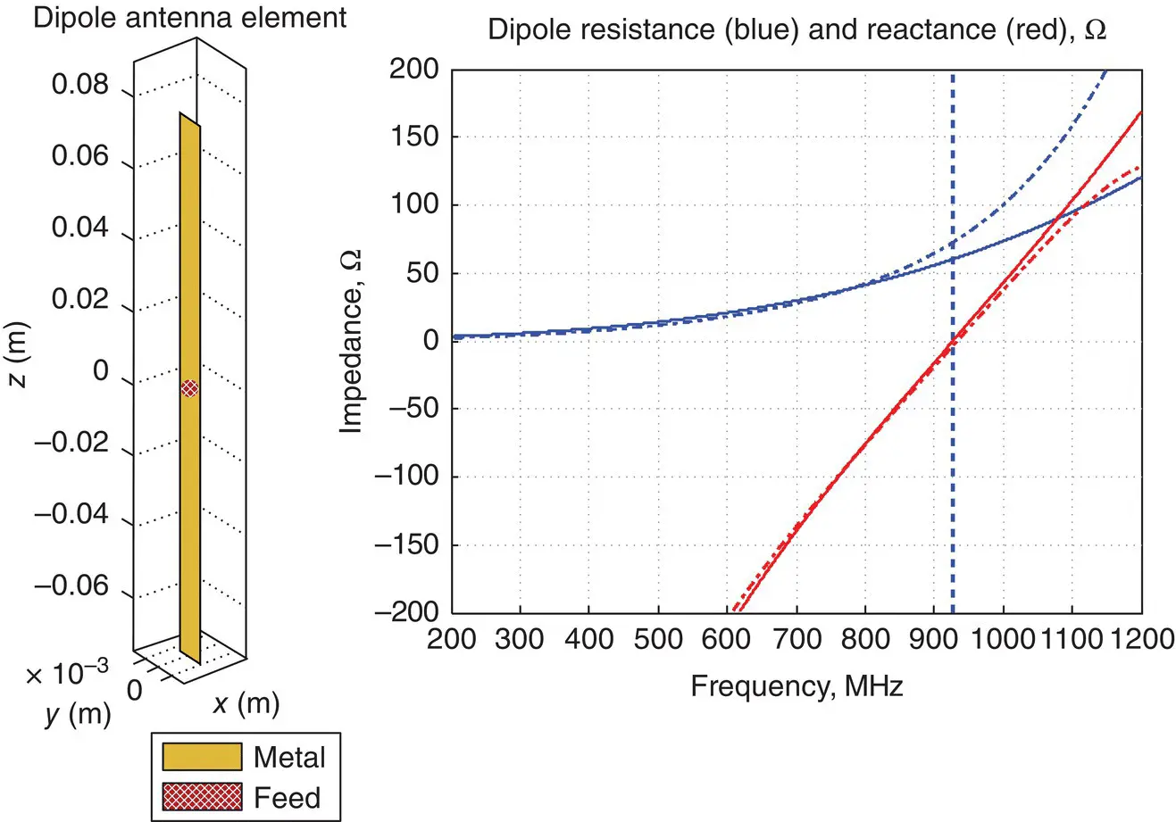
Figure 1.6 Dipole antenna impedance in the vicinity of its first (series) resonance. The dashed line shows the resonant frequency. The solid curves show the analytical antenna impedance. The dash‐dot curves show the simulated antenna impedance.