Machine Learning for Healthcare Applications
Здесь есть возможность читать онлайн «Machine Learning for Healthcare Applications» — ознакомительный отрывок электронной книги совершенно бесплатно, а после прочтения отрывка купить полную версию. В некоторых случаях можно слушать аудио, скачать через торрент в формате fb2 и присутствует краткое содержание. Жанр: unrecognised, на английском языке. Описание произведения, (предисловие) а так же отзывы посетителей доступны на портале библиотеки ЛибКат.
- Название:Machine Learning for Healthcare Applications
- Автор:
- Жанр:
- Год:неизвестен
- ISBN:нет данных
- Рейтинг книги:5 / 5. Голосов: 1
-
Избранное:Добавить в избранное
- Отзывы:
-
Ваша оценка:
Machine Learning for Healthcare Applications: краткое содержание, описание и аннотация
Предлагаем к чтению аннотацию, описание, краткое содержание или предисловие (зависит от того, что написал сам автор книги «Machine Learning for Healthcare Applications»). Если вы не нашли необходимую информацию о книге — напишите в комментариях, мы постараемся отыскать её.
Since this book is intended to be useful to a wide audience, students, researchers and scientists from both academia and industry may all benefit from this material. It contains a comprehensive description of issues for healthcare data management and an overview of existing systems, making it appropriate for introductory and instructional purposes. Prerequisites are minimal; the readers are expected to have basic knowledge of machine learning.
This book is divided into 22 real-time innovative chapters which provide a variety of application examples in different domains. These chapters illustrate why traditional approaches often fail to meet customers’ needs. The presented approaches provide a comprehensive overview of current technology. Each of these chapters, which are written by the main inventors of the presented systems, specifies requirements and provides a description of both the chosen approach and its implementation. Because of the self-contained nature of these chapters, they may be read in any order. Each of the chapters use various technical terms which involve expertise in machine learning and computer science.
Machine Learning for Healthcare Applications — читать онлайн ознакомительный отрывок
Ниже представлен текст книги, разбитый по страницам. Система сохранения места последней прочитанной страницы, позволяет с удобством читать онлайн бесплатно книгу «Machine Learning for Healthcare Applications», без необходимости каждый раз заново искать на чём Вы остановились. Поставьте закладку, и сможете в любой момент перейти на страницу, на которой закончили чтение.
Интервал:
Закладка:
3.3.3 Kernel Support Vector Machine (Sigmoid)
The separable data with non-linear attributes cannot be tackled by a simple Support Vector Machine algorithm due to which we use a modified version of it called Kernel Support Vector Machine. Essentially in K-SVM it presents the data from a non-linear lower dimension to a linear higher dimension form as such that the attributes belonging to variable classes are assigned to different dimensions. We use a simple Python-SciKit Learn Library to implement and use K-SVM.
For training purposes, we use the SVC class of the library. The difference is in the values for the Kernel parameters of SVC class. In simple SVM’s we use “Linear” for Kernel parameters but in K-SVM we use Gaussian, Sigmoid, Polynomial, etc. wherein we have used Sigmoid.
The only limitation observed in our case is that though this method achieves the highest accuracy but not up to the mark. Hence more advanced models like Deep Learning may be applied in near future for more concrete results.
3.3.4 Random Decision Forest Classifier
It is a variant of supervised machine learning algorithm founded on the schematic of ensembled learning. Ensemble learning is an algorithm where you join multiple or single algorithm into multiple types of algorithms of multiple or same variant to create a complex and advanced prediction model. It also combines many algorithms of same variant as decision trees, forest trees, etc. so the name “Random Forest”. It is used for regression and classification tasks.
The way it works is it picks a part of the dataset and builds a decision tree on these records, and after selection of number of trees you want this process is repeated. Each tree represents the prediction in that category for which the new record belongs. The only limitation here is that there forte lies in their complexity and for that we need substantial computing resources when huge number of decision trees can be brought together which in turn will better train themselves.
3.4 System Setup & Design
We have used an Emotiv EPOC+ biosensor device for capturing Neuro-Signals in the following manner. Figure 3.1represents the channels on the brain from signals collected and the equipment used for collection. The signals are collected from 14 electrodes positioned at “AF3, AF4, F3, F4, F7, F8, FC5, FC6, O1, O2, P7, P8 T7 and T8” according to International 10–20 system viewed in the figure below. There are reference electrodes positioned above ears at CMS and DRL. By default, the device has a sampling frequency of 2,048 Hz which we have down-sampled to 128 Hz per channel. The data acquired is transmitted using Bluetooth connectivity to a system. Before every sample collection sensor felt pads are rubbed with saline, connected via the Bluetooth USB and charged after with a USB cable as shown in the figure below.
The device is placed on the participants and then showed a particular set of common usage items for the purpose of our experiment, during which all the EEG activity is recorded and later on they are asked to label their choice of purchase amongst each set of products i.e. 1 among 3 items of from each set of products. The process diagram can be seen below in Figure 3.2.
After the data collection, the signals are preprocessed, and some features are extracted using wavelet transformation method and then the classification models were run on the resultant as mentioned before. A part of the data was is preprocessed and decomposed to test the training model. The labeling was done majorly into Like/Dislike.
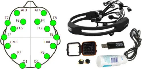
Figure 3.1 Brain map structure and Equipment used.
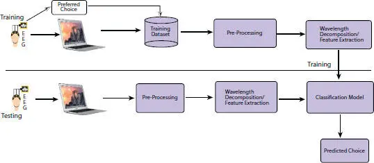
Figure 3.2 Workflow diagram.
3.4.1 Pre-Processing & Feature Extraction
We shall discuss how we used S-Golay filter to even out the signals and then DWT based wave-let analysis to extract features from Neuro-signals.
3.4.1.1 Savitzky–Golay Filter
In layman words [24] if we try to understand this filter, it is a polynomial based filter in which least square polynomial method find out the filtered signals with combinedly evaluating the neighbor signals. It can be computed for a signal such as S j= f(t j), (j = 1, 2, …, n) by following Equation (3.3).
(3.3) 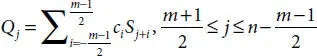
Here, ‘m’ is frame span, c iis no. of convolution coeffs. and Q is the resultant signal. ‘m’ is used to calculate instances of c iwith a polynomial. In our case, this was used to smoothen Neuro-signals by a frame size of 5 with a polynomial of degree 4.
3.4.1.2 Discrete Wavelet Transform
In layman words, it is used to convert incoming signal into sequences of smaller waves using multi-stage decomposition. This enables us to analyze multiple oscillatory signals in an approximation and detail coefficient form. Figure 3.3has shown the decomposing structural of brain neuron signals when it is preprocessed using low & high filtering methods. Low filter pass method (L) removes high voltage fluctuations and saves slow trends. These in turn provide approximation (A) of the signal. High pass filter method (H) eliminates the slow trends and saves the high voltage fluctuations. The resultant of (H) provides us with detail coefficient (D) which is also known as Wavelet coefficient. The Wavelet function is shown in Equations (3.4)and (3.5).
(3.4) 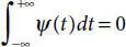
(3.5) 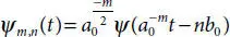
Here ‘a’ and ‘b’ are scaling parameter and translation parameter containing discrete values. ‘m’ is frequency and ‘n’ is time belonging to Z. The computation of (A) and (D) is shown in scaling function (3.6)and wavelet function (3.7).
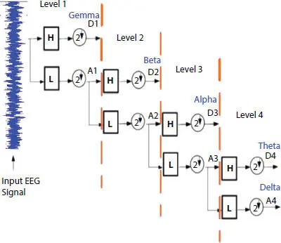
Figure 3.3 DWT schematic.
(3.6) 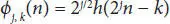
(3.7) 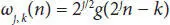
Here, φ j,k(n) is the scaling function belonging to (L) and ω j,k(n) is the wavelet function belonging to (H), M is length of signal, n is the discrete variable lies between 0 and M − 1, J = log 2(M), with k and j taking values from {0 – J − 1}. The values of A iand D iare computed below by Equations (3.8)and (3.9).
(3.8) 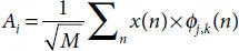
(3.9) 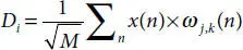
Интервал:
Закладка:
Похожие книги на «Machine Learning for Healthcare Applications»
Представляем Вашему вниманию похожие книги на «Machine Learning for Healthcare Applications» списком для выбора. Мы отобрали схожую по названию и смыслу литературу в надежде предоставить читателям больше вариантов отыскать новые, интересные, ещё непрочитанные произведения.


Обсуждение, отзывы о книге «Machine Learning for Healthcare Applications» и просто собственные мнения читателей. Оставьте ваши комментарии, напишите, что Вы думаете о произведении, его смысле или главных героях. Укажите что конкретно понравилось, а что нет, и почему Вы так считаете.