Anand K. Verma - Introduction To Modern Planar Transmission Lines

Figure (2.9a)shows that the maximum available power from a source is computed by directly connecting the load to it. The average power supplied to the load is

(2.1.113)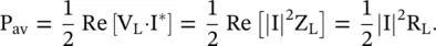

The load current is

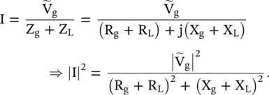
Therefore, the average power supplied to the load is

(2.1.114)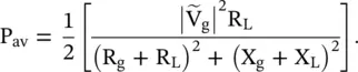

Under the conjugate matching , X L= −X gand R L= R g, the average power supplied to load is maximum:

(2.1.115)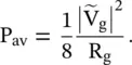

This is the maximum power available from a generator under the matching condition and delivered to a load R L. At this stage, the maximum power delivered to a load is computed in the absence of the transmission line. For a matched terminated lossless line, the maximum available power from the source is delivered to the load. It is examined below.

The voltage and current waves on a line under no reflection case are

(2.1.116)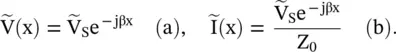

The average power on the line is

(2.1.117)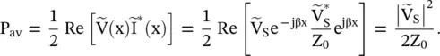

On a lossless line, the average power is independent of the distance x from a source. Physically it makes a sense, as the same amount of power flows at any location on the line. Under the matched load termination, Z L= Z 0, the input impedance at the source end is Z 0itself. It is shown in Fig (2.9b). The sending end voltage at the input port – aa of a transmission line is

(2.1.118)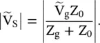

The maximum power is transferred from a generator to the transmission line under the matching condition, R g= Z 0. The maximum available power from the generator to feed the line is given by equation (2.1.115). It is identical to the power determined from equation (2.1.117), as .

If the line is not terminated in its characteristic impedance, then a reflection takes place at the load end. The reflected wave travels from the load toward the generator given by

(2.1.119)

The average power in the reflected wave is

(2.1.120)

However, at the load end amplitude of the reflected voltage wave is V −= Γ LV +; where . Therefore, the average reflected power on the line is

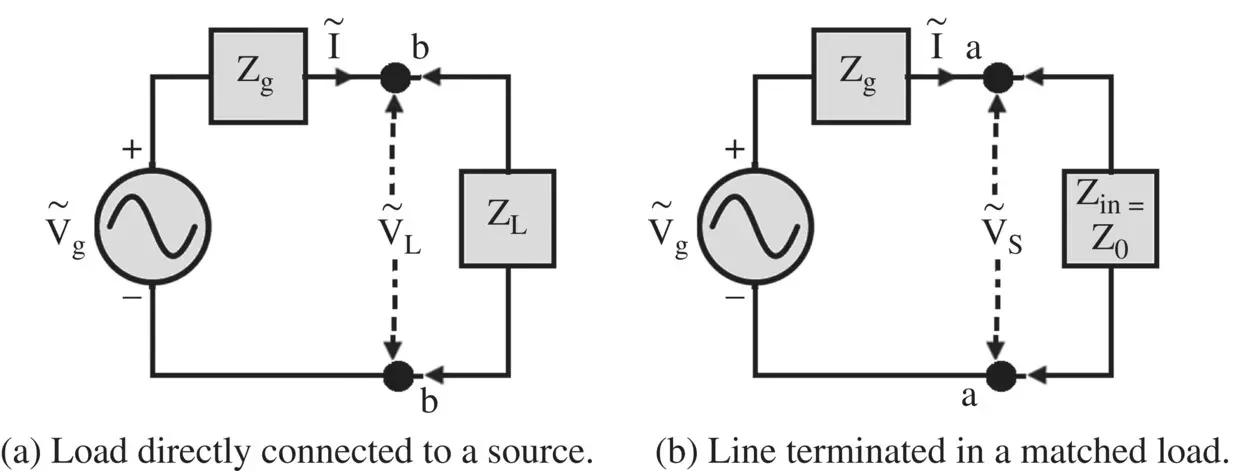
Figure 2.9 Load connections to a source.

(2.121)

The negative sign (−) shows that the reflected power travels from the load toward the source. Finally, under the mismatched load, the power delivered to the load is obtained from equations (2.1.117)and (2.1.121)

(2.1.122)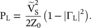

For a lossless line, the power balance is written as follows:

(2.1.123)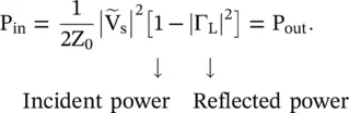

In equation (2.1.123), input power P inat the input port – aa of the line enters into the line. It is supplied by a source. The output power P outis the power supplied to the load.

This section extends the solution of the voltage wave equation to the multisection transmission line [B.8, B.16]. Next, the voltage responses are obtained for the shunt connected current source, and also the series‐connected voltage source, at any location on a line. This treatment is used in chapters 14and 16for the spectral domain analysis of the multilayer planar transmission lines.

Figure (2.10a)shows a multisection transmission line, consisting of the N number of line sections. Each line section has different lengths (d 1, d 2,…,d N), different characteristic impedances (Z 01, Z 02,…,Z 0N), or different characteristic admittances (Y 01, Y 02,…,Y 0N) and different propagation constants (β 1, β 2, …, β N). At each junction of two dissimilar lines, the voltage wave reflection occurs with the reflection coefficient Γ 1, Γ 2, …, Γ N. At each junction, the input admittance of all succeeding line sections appears as a load. The input admittances at junctions (x 1, x 2, …, x N)are . The distances of the junctions are measured from the origin that is located on the left‐hand side. The input terminals of line sections 1,2,…,N − 1 are located at the junctions (x 0,x 1, x 2,…,x N). The voltage source V sis located at the input of the first line section. The last line section is terminated in the load Z L= 1/Y L.

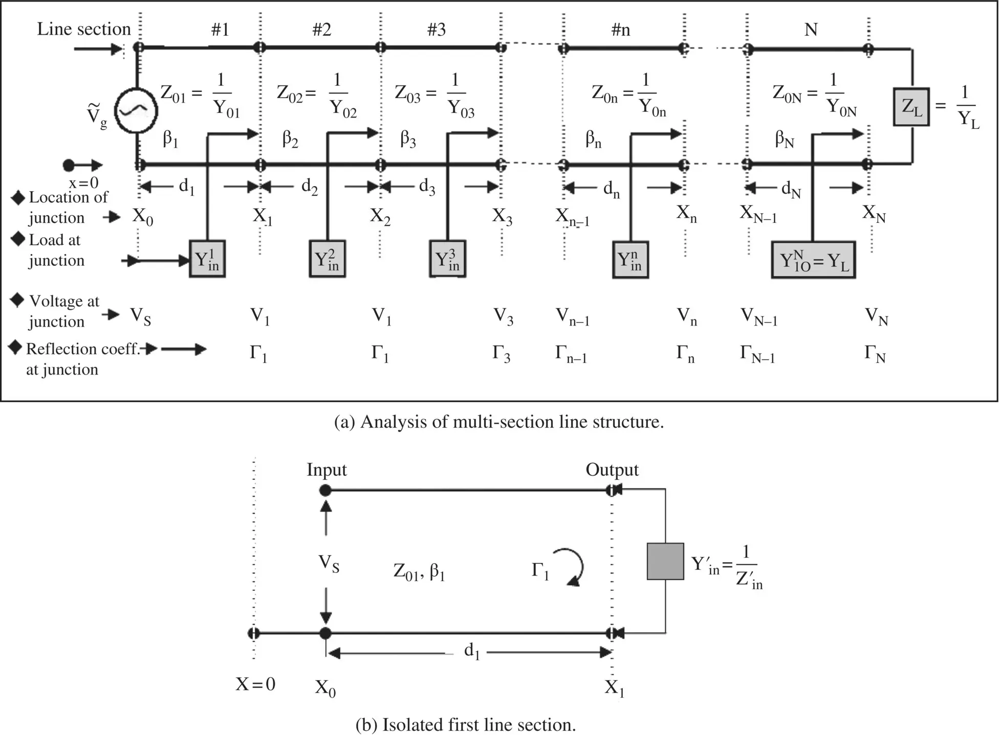
Figure 2.10 The multisection transmission line.

The objective is to find the voltage at each junction of the multisection line. Further, the voltage distribution on each line section is determined due to the input voltage .

The solutions for the voltage and current wave equations involve four constants. The constants of the current wave are related to two constants of the voltage wave through the characteristic impedance of a line. Out of two constants of the voltage wave, one is expressed in terms of the reflection coefficient at the load end; that itself is expressed by the characteristic impedance and the terminated load impedance. The reflection coefficient can also be expressed by the characteristic admittance and the terminated load admittance. The second constant is evaluated by the source condition at the input end. Figure (2.10b)shows the first isolated line section. The voltage and current waves, with respect to the origin at the load end x 1, on the line section (x 0≤ x ≤ x 1) are written from equation (2.1.88):