Anand K. Verma - Introduction To Modern Planar Transmission Lines

Figure (2.8a)shows a section of the transmission line having a length ℓ. It is fed by a voltage source, with Z ginternal impedance. The general solutions for the line voltage and line current of the wave equation (2.1.37)are

(2.1.55)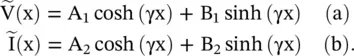

At any section on the line, its characteristic impedance Z 0relates the line voltage and line current . So the constants A 2, B 2are related to the constants A 1and B 1. In Fig (2.8a), the point P on the line is located at a distance x from the source end , i.e. at a distance d = (ℓ − x) from the load end . The load is located at d = 0, and the source is located at d = − ℓ. The , and are the input voltage and the input current at the port‐aa, i.e at x = 0. At x = ℓ, i.e. 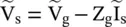at the port‐bb, and are the load end voltage and current, respectively. The ideal voltage generator has the internal impedance, Z g= 0, i.e. . The phasor form of the line current, from equations (2.1.32b)and (2.1.55a), is written below:

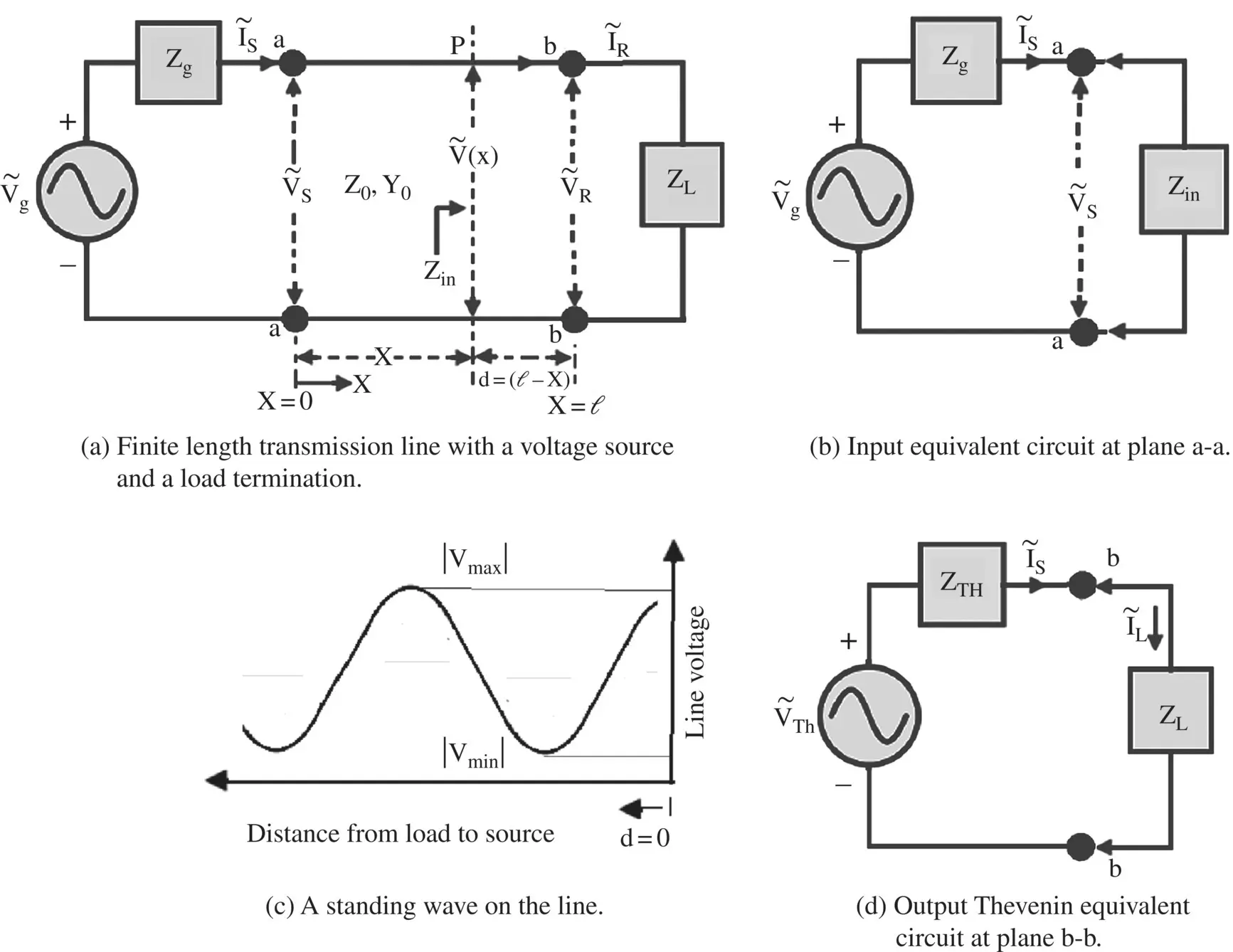
Figure 2.8 Transmission line circuit. The distance x is measured from the source end; whereas the distance d is measured from the load.

(2.1.56)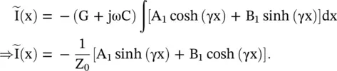

On comparing the coefficients of sinh(γx) and cosh(γx), of equations (2.1.55b)and (2.1.56), two constants A 2and B 2are determined:

(2.1.57)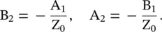

The phasor line voltage and line current are written as follows:

(2.1.58)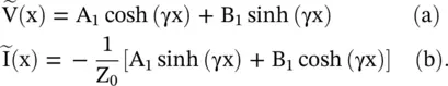

The constants A 1and B 1are determined by using the boundary conditions at input x = 0 and output x = ℓ.

At x = 0, the line input voltage is , giving the value of A1:(2.1.59)

At the receiving end, x = ℓ, the load end voltage and current are

(2.1.60)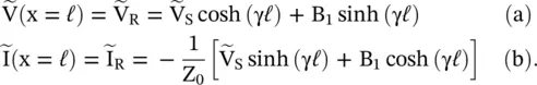

At x = ℓ, i.e. at the receiving end, the voltage across load ZL is(2.1.61)

The constant B 1is evaluated on substituting and , from equation (2.1.60), in the above equation:

(2.1.62)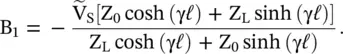

On substituting constants A 1and B 1in equation (2.1.58a), the expression for the line voltage at location P, from the source or load end, is

(2.1.63)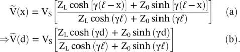

Similarly, the line current at the location P is obtained as follows:

(2.1.64)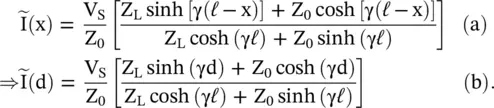

At any location P on the line, the load impedance is transformed as input impedance by the line length d = (ℓ − x):

(2.1.65)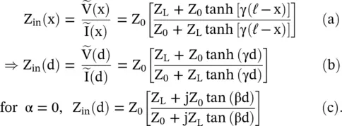

Equations (2.1.65a,b)take care of the losses in a line through the complex propagation constant, γ = α + jβ. However, for a lossless line α = 0, γ = jβ and the hyperbolic functions are replaced by the trigonometric functions shown in equation (2.1.65c). It shows the impedance transformation characteristics of d = λ/4 transmission line section.

Equations (2.1.63)and (2.1.64)could be further written in terms of the generator voltage for the case, Z g≠ 0. Figure (2.8b)shows that at the source end x = 0, the load appears as the input impedance Z in. The sending end voltage is obtained as follows:

, where .

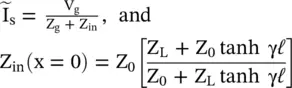(2.1.66)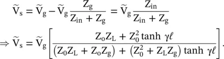

The line voltage, in terms of , and Z L, is obtained on substituting equation (2.1.66)in equation (2.1.63):