Modern Trends in Structural and Solid Mechanics 1
Здесь есть возможность читать онлайн «Modern Trends in Structural and Solid Mechanics 1» — ознакомительный отрывок электронной книги совершенно бесплатно, а после прочтения отрывка купить полную версию. В некоторых случаях можно слушать аудио, скачать через торрент в формате fb2 и присутствует краткое содержание. Жанр: unrecognised, на английском языке. Описание произведения, (предисловие) а так же отзывы посетителей доступны на портале библиотеки ЛибКат.
- Название:Modern Trends in Structural and Solid Mechanics 1
- Автор:
- Жанр:
- Год:неизвестен
- ISBN:нет данных
- Рейтинг книги:4 / 5. Голосов: 1
-
Избранное:Добавить в избранное
- Отзывы:
-
Ваша оценка:
Modern Trends in Structural and Solid Mechanics 1: краткое содержание, описание и аннотация
Предлагаем к чтению аннотацию, описание, краткое содержание или предисловие (зависит от того, что написал сам автор книги «Modern Trends in Structural and Solid Mechanics 1»). Если вы не нашли необходимую информацию о книге — напишите в комментариях, мы постараемся отыскать её.
Modern Trends in Structural and Solid Mechanics 1 — читать онлайн ознакомительный отрывок
Ниже представлен текст книги, разбитый по страницам. Система сохранения места последней прочитанной страницы, позволяет с удобством читать онлайн бесплатно книгу «Modern Trends in Structural and Solid Mechanics 1», без необходимости каждый раз заново искать на чём Вы остановились. Поставьте закладку, и сможете в любой момент перейти на страницу, на которой закончили чтение.
Интервал:
Закладка:
[1.5a] 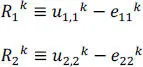
[1.5b] 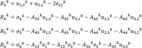
[1.5c] 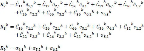
In equations [1.5b]and [1.5c], the coefficients Aijk represent the elasticities of the k thlayer material, with respect to the layer material principal axes rotated with respect to the analysis coordinate system (see Figure 1.1). The  quantities are found by expressing the in-plane stresses and transverse strains in terms of the transverse stresses and in-plane strains (i.e. the layerwise continuous variables) from equations [1.2]and [1.3](see Moleiro et al . 2011). It should be highlighted that in-plane strains have been incorporated into the mixed formulation, in order to recast the governing equations into first-order form, which allows the use of C 0basis functions for the interpolation of unknown variables, discussed later. While this increases the number of unknowns to solve for, the advantage is that continuity of surface tractions and displacements at layer interfaces can now be enforced.
We note that Rka = 0, a = 1, 2, …, 9 are the nine equations for the nine unknowns in sk. Recall that there are three boundary conditions prescribed at each bounding face of the lamina. Generally, the top and the bottom faces of a lamina have prescribed tractions,  , on them, and edges x = 0, a and y = 0, b have a combination of fi and ui , where
  and
and  are the known function of the in-plane coordinates. For example, at a clamped edge,
  , and at a free edge,
  . At a simply supported edge x = 0, we set
[1.6] 
Equation [1.6] 3is equivalent to a null in-plane normal stress at the edge x = 0. Since in-plane stresses are not directly computed in the present formulation, we write this boundary condition residual in terms of the variables in sas
[1.7] 
which also uses the constitutive relation in equation [1.4]. Thus, for each one of the six bounding faces, we will have three residuals that we denote by R 10through R 27.
We define the functional, J , in terms of the residuals, with contributions from each material layer as
[1.8] 
We note that the repeated index a goes from 1 to 9, and the second surface integral is for the six bounding surfaces of a lamina, and in it, Rbk (b = 10, 11, …, 27) are residuals for the boundary conditions of the k thlayer. In equation [1.8], Ω denotes either the in-plane domain of the plate or one of its edge surfaces, hk is the thickness of the kth layer. In evaluating integrals with respect to x 3, elasticities of the individual layer are considered.
Each element of the nine-dimensional vector skis expressed as the product of complete Lagrange polynomials of degrees N 1, N 2and N 3in x 1, x 2and x 3defined as follows:
[1.9] 
[1.10] 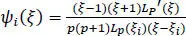
Note that equation [1.9]has 9 x N 1x N 2x N 3unknowns, Saijk , for each layer. In equation [1.10], the basis function ψi is written in natural coordinates, ξ , and in terms of the Pth -order Lagrange polynomial LP ( ξ ) and its derivative, indicated by the prime symbol. The quantity ξi is a root of the equation P n( ξ ) = 0, where P nis a Legendre polynomial of order n . Basis functions given in [1.10]are associated with Gauss–Lobatto points. Substitution from equation [1.10]into equation [1.9], the result into equation [1.8], and the numerical evaluation of the integral by using the Gauss–Lobatto quadrature rule of order Pn in the three directions, gives J as a function of Saijk . We deduce the needed linear algebraic equations by setting
[1.11] 
We realize that expressions for the residuals have different units. When equation [1.11]is written as KA= F, it is likely that the use of non-dimensional variables throughout the chapter will improve the condition number of the matrix Kand reduce error. However, we have not tried this. A feature of the equations derived from [1.11]using basis functions of type [1.10]is that they are insensitive to shear-locking effects, which means that reduced integration is not needed in the thickness direction.
We note that the above formulation holds for a laminate, when the continuity of variables u 1, u 2, u 3, σ 4, σ 5, σ 6, e 1, e 2, e 3is enforced by adding the appropriate residuals in equation [1.8]or using a layerwise theory. Here, we use a layerwise theory, where the contribution from each layer is included in the summation in equation [1.8]and the continuity of the variables in sat each layer interface is ensured.
1.3. Results and discussion
1.3.1. Verification of the numerical algorithm
To verify the algorithm and to establish the accuracy of computed results, we study the problem analytically analyzed by Pagano (1969). It involves a four-layered [0/90/90/0] simply supported square laminate of side length a , with the sinusoidal surface traction
[1.12] 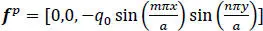
Интервал:
Закладка:
Похожие книги на «Modern Trends in Structural and Solid Mechanics 1»
Представляем Вашему вниманию похожие книги на «Modern Trends in Structural and Solid Mechanics 1» списком для выбора. Мы отобрали схожую по названию и смыслу литературу в надежде предоставить читателям больше вариантов отыскать новые, интересные, ещё непрочитанные произведения.


Обсуждение, отзывы о книге «Modern Trends in Structural and Solid Mechanics 1» и просто собственные мнения читателей. Оставьте ваши комментарии, напишите, что Вы думаете о произведении, его смысле или главных героях. Укажите что конкретно понравилось, а что нет, и почему Вы так считаете.