Mantle Convection and Surface Expressions

Changes in the continuity and shape of upwelling and downwelling features have been identified in both global and regional tomographic models. The whole‐mantle waveform tomographic model SEMUCB‐WM1 (French and Romanowicz, 2014) reveals striking lateral deflections of upwellings beneath several active hotspots. In particular, the imaged plume conduit beneath St. Helena appears to be deflected 1,000–650 km, in contrast to its more vertical shape in the lower mantle below 1,000 km and in the upper mantle and transition zone (French and Romanowicz, 2015). While St. Helena provides perhaps the most striking example, there are also possible deflections near 1,000 km beneath the Canaries and Macdonald (French and Romanowicz, 2015). Regional tomography of the North Atlantic shows some evidence of deflection of the Iceland plume above 1,000 km depth (Rickers et al., 2013), though this is not seen in all regional and global models (French and Romanowicz, 2015; Yuan and Romanowicz, 2017). Regional tomography indicates that the Yellowstone plume is laterally shifted near 1,000 km (Nelson and Grand, 2018). Slabs imaged in the global P wave model GAP‐P4 (Obayashi et al., 2013; Fukao and Obayashi, 2013) appear to stagnate within or below the mantle transition zone. The Northern Mariana slab is imaged as a nearly horizontal feature above 1,000 km, the Java slab is stagnant or less steeply inclined above 1,000 km, and the Tonga slab is imaged as a horizontal fast anomaly above 1,000 km (Fukao and Obayashi, 2013). This behavior is not universal; in Central America, there is no evidence for slab ponding or stagnation, and many slabs in the Western Pacific and South America are imaged above 650 km depth.

Seismic scatterers have been identified in the mid‐mantle, and their depth‐distribution peaks near 1,000 km. Using P ‐to‐ S receiver function stacks, Jenkins et al. (2016) located scatterers beneath Europe, Iceland, and Greenland. The scatterers are distributed at depths of ∼800–1400 km, with a peak near 1,000 km. In global surveys of seismic reflectors, scatterers are observed in all regions with data coverage, and with no clear association to tectonic province or subduction history (Waszek et al., 2018; Frost et al., 2018). The global distribution of reflectors imaged by Waszek et al. (2018) is quite broadly distributed across the depth range of 850–1300 km with a peak close to 875 km depth. Changes in the distribution of small‐scale heterogeneity are also supported by analyses of the spectra of tomographic models. A decrease in the redness in mantle tomographic models occurs below 650 km, coincident with the observations of short‐wavelength scattering features, stagnant slabs, and deflected upwellings.

The observational evidence for changes in mantle structure from long‐wavelength radial correlation, the behavior of upwellings and downwellings, and the depth‐ and lateral‐distribution of short wavelength scattering features suggests the possibility of changes in mantle properties and processes in the mid mantle. Several mechanisms have been proposed for such a change, including a change in viscosity (Rudolph et al., 2015) or a change in composition (Ballmer et al., 2015). In the remainder of this chapter, we present new analyses of mantle tomographic models with an eye toward understanding which features in the tomographic models give rise to the changes in the long‐wavelength radial correlation structure. Next, we use 3D spherical geometry mantle convection models to assess the implications of different mantle viscosity structures for the development of large‐scale structure. Finally, we examine previous and new inferences of the mantle viscosity profile, constrained by the long‐wavelength geoid.

We compare the results of the geodynamic modeling with the characteristics of four recent global tomographic V Smodels that differ in data selection, theoretical framework, and model parameterization and regularization choices. SEMUCB‐WM1 (French and Romanowicz, 2014) is a global anisotropic shear‐wave tomographic model based on full‐waveform inversion of three‐component long‐period seismograms, divided into wavepackets containing body waves and surface waves including overtones. Accurate waveform forward modeling is achieved using the spectral element method (Capdeville et al., 2005), 2D finite frequency kernels are computed using nonlinear asymptotic coupling theory (Li and Romanowicz, 1995), and the tomographic model is constructed by iterating using the quasi‐Newton method. SEISGLOB2 (Durand et al., 2017) is an isotropic shear‐wave model constrained by data sensitive primarily to V SVstructure–spheroidal mode splitting functions, Rayleigh wave phase velocity maps, and body wave traveltimes. The inverse problem is fully linearized, with sensitivity of normal mode and Rayleigh wave data computed using first order normal mode perturbation theory, and traveltime data using ray theory, both computed in a reference spherically symmetric model. GLAD‐M15 (Bozdağ et al., 2016) is a global tomographic model that, like SEMUCB‐WM1, aims to fit full, three‐component seismic waveforms. Once again, the spectral element method (Komatitsch and Tromp, 2002) enables accurate forward modeling, while 3D finite frequency kernels are computed using the adjoint method at each iteration. GLAD‐M15 uses S362ANI (Kustowski et al., 2008) as a starting model and carries out an iterative conjugate gradient refinement of the 3D velocity structure to match observations while accounting for the full nonlinearity of the sensitivity of the misfit function to earth structure. The fourth model, S362ANI+M (Moulik and Ekström, 2014), is a global model based on full‐spectrum tomography, which employs seismic waveforms and derived measurements of body waves (∼1–20s), surface waves (Love and Rayleigh, ∼20–300s), and normal modes (∼250–3300s) to constrain physical properties – seismic velocity, anisotropy, density, and the topography of discontinuities – at variable spatial resolution. The inverse problem is solved iteratively and jointly with seismic source mechanisms, using sensitivity kernels that account for finite‐frequency effects for the long‐period normal modes, along‐branch coupling for waveforms and ray theory for body‐wave travel times and surface‐wave dispersion. Model SEISGLOB2 was obtained as spatial expansions of Voigt V Sin netcdf format from the IRIS Data Management Center ( http://ds.iris.edu/ds/products/emc‐earthmodels/http://ds.iris.edu/ds/products/emc‐earthmodels/). S362ANI+M was provided in netcdf format on a two‐degree grid and at 25 depths. GLAD‐M15 was provided on a degree‐by‐degree grid and at 132 depths by the authors (Bozdagˇ, pers. comm .). Model SEMUCB‐WM1 was obtained from the authors’ web page and evaluated using the model evaluation tool a3don a degree‐by‐degree grid at 65 depths.

The tomographic models were expanded into spherical harmonics to calculate power spectra and to facilitate wavelength‐dependent comparisons among models. First, at each depth, models were resampled using linear interpolation onto 40,962 equispaced nodes, providing a uniform resolution equivalent to 1 × 1 equatorial degree. Spherical harmonic expansions were carried out using the slepian MATLAB routines (Simons et al., 2006). Spherical harmonic coefficients were computed using the 4 π ‐normalized convention, such that the spherical harmonic basis functions Y lmsatisfy 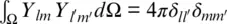where Ω is the unit sphere. The power per degree and per unit area was computed as