Mantle Convection and Surface Expressions

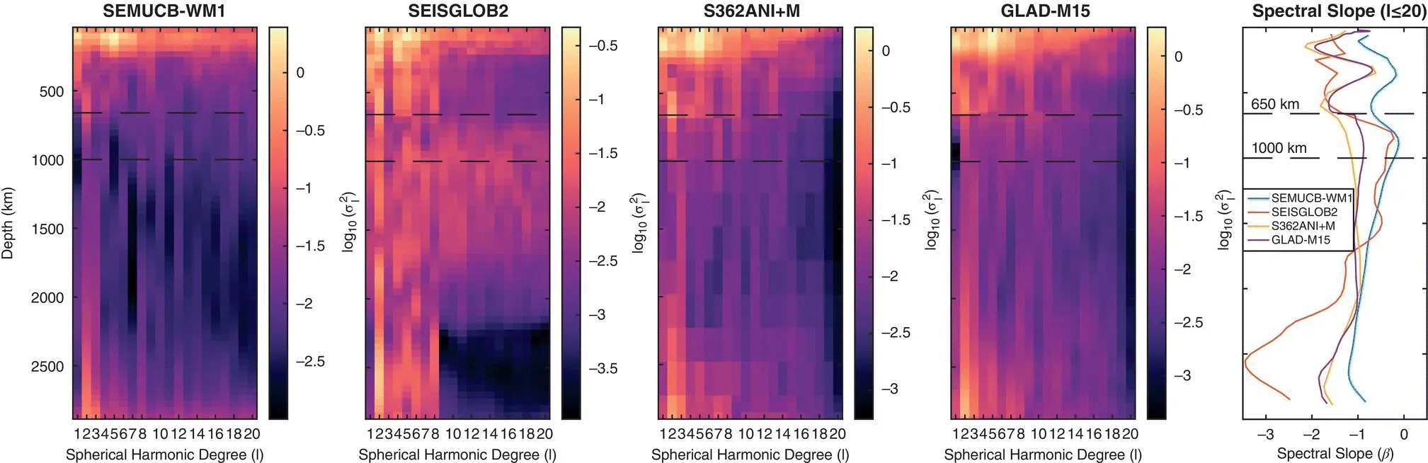
Figure 1.5 Power spectra of four recent global V Stomographic models. Because our focus is on long‐wavelength structure, and to ensure a more equitable comparison, we show only spherical harmonic degrees 1–20, though SEMUCB‐WM1, SEISGLOB2, and GLAD‐M15 contain significant power at shorter wavelengths. At the right, we show spectral slopes (defined in the text) for the four models. Here, increasingly negative values indicate a concentration of power in longer wavelengths/lower spherical harmonic degrees.

Figure 1.3shows radial correlation plots for the four tomographic models. Here, the spherical harmonic expansions are truncated at degrees 2 (lower left triangle) and 4 (upper right triangle). At degrees 1–2 and 1–4, both SEMUCB‐WM1 and SEISGLOB2 show a clear change in the correlation structure near 1,000 km depth. On the other hand, S362ANI+M and GLAD‐M15 both show a change in correlation structure at 650 km.

We compared the character of heterogeneity in the geodynamic models with mantle tomography by calculating the power spectrum and spectral slope of each of the five geodynamic models. Because the depth‐variation of power in the geodynamic models does not have as straightforward an interpretation as the V Spower spectra shown for tomographic models, we focus on the spectral slope of the geodynamic models, shown in Figure 1.4. We computed correlation coefficients between each of the geodynamic models and SEMUCB‐WM1, shown in Figure 1.4C.

For both of the tomographic models used to infer mantle viscosity, we carried out viscosity inversions ( Figure 1.6) constrained by spherical harmonic degree 2 only, degrees 2 and 4 only, and degrees 2–7. The viscosity profiles are quite similar, regardless of which spherical harmonic degrees are used to constrain the inversion. However, we observe an increase in the overall complexity of the viscosity profile as more spherical harmonic degrees are included, as well as a tendency towards developing a low‐viscosity region below the 650 km discontinuity (red curves in Figure 1.6), considered in the context of parsimonious inversions, this tendency toward increased complexity can be attributed to the progressively greater information content of the data. The posterior ensembles from the viscosity inversions contain significant variability among accepted solutions, and the solid lines in Figure 1.6indicate the log‐mean value of viscosity present in the ensemble at each depth while the shaded regions enclose 90% of the posterior solutions. We note that while the individual solutions in the posterior ensemble produce an acceptable misfit to the geoid, the ensemble mean itself may not. Therefore, potential applications in the future need to account for all samples of viscosity models in our ensemble rather than employ or evaluate the ensemble mean in isolation.

The recent tomographic models considered here show substantial discrepancies in the large‐scale variations within the mid mantle. The low overall RMS of heterogeneity (with the consequent small contribution to data variance) and a reduction in data constraints at these depths (e.g., normal modes, overtone waveforms) exacerbates the relative importance of a priori information (e.g., damping) in some tomographic models. The RCF plots shown in Figure 1.3show that even at the very long wavelengths characterized by spherical harmonic degrees 1–2 and 1–4, there is rapid change in the RCF near 1,000 km in SEMUCB‐WM1 and SEISGLOB2. On the other hand, S362ANI+M and GLAD‐M15 both show more evidence for a change in structure near 1,000 km at degrees 1–2 but closer to the 650 km discontinuity for degrees up to 4. In order to understand the changes in the RCF, spatial expansions of the structures in the four tomographic models are shown for degrees 1–4 and at depths within the lithosphere, transition zone, and lowermost mantle are shown in Figure 1.2. We previously examined the long‐wavelength structure of SEMUCB‐WM1 and suggested that the changes in its RCF at 1,000 km depth are driven primarily by the accumulation of slabs in and below the transition zone in the Western Pacific (Lourenço and Rudolph, in review).

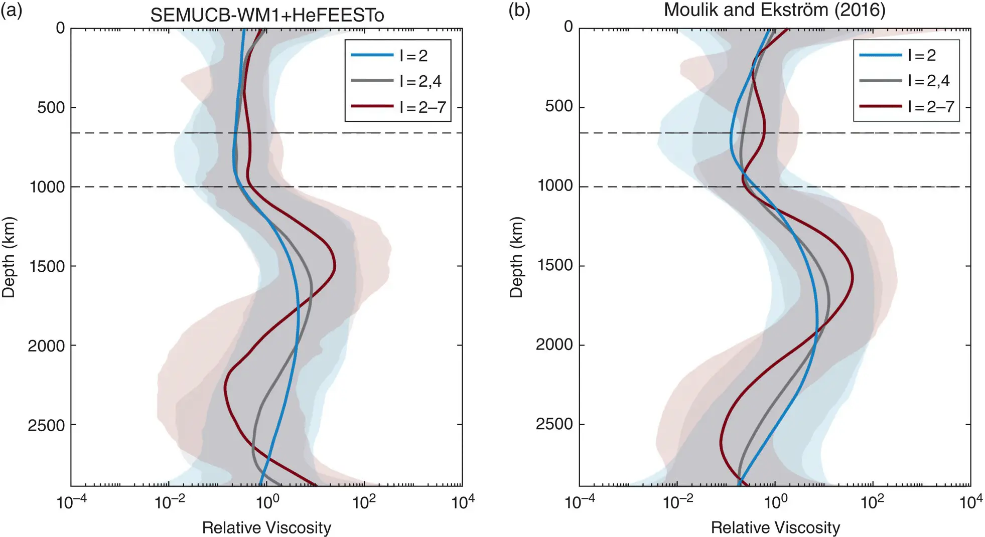
Figure 1.6 Results from transdimensional, hierarchical, Bayesian inversions for the mantle viscosity profile, using two different models for density. (a) Density was scaled from Voigt V Svariations in SEMUCB‐WM1 using a depth‐dependent scaling factor computed using HeFESTo (Stixrude and Lithgow‐Bertelloni, 2011). (b) Density variations from a joint, whole‐model mantle of density and seismic velocities (Moulik and Ekström, 2016)

The shift in pattern of mantle heterogeneity within and below the transition zone is influenced by changes in the large‐scale structure of plate motions. In Figure 1.7, we show the long‐wavelength structure of plate motions at 0, 100, and 200 Ma. We expanded the divergence component of the plate motion model by Matthews et al. (2016) using spherical harmonics and show only the longest‐wavelength components of the plate motions. This analysis is similar in concept to the multipole expansion carried out by Conrad et al. (2013) to assess the stability of long‐wavelength centers of upwelling, as a proxy for the long‐term stability of the LLSVPs. These long‐wavelength characteristics of the plate motions need to be interpreted with some caution because the power spectrum of the divergence of plate motions is not always dominated by long‐wavelength power, and power at higher degrees may locally erase some of the structure that overlaps with low spherical harmonic degrees (Rudolph and Zhong, 2013). However, for the present day ( Figure 1.7, right column), the long‐wavelength divergence field does show a pattern of flow with centers of long‐wavelength convergence centered beneath the Western Pacific and beneath South America, where most of the net convergence is occurring. On the other hand, at 100 and 200 Ma, the pattern of long‐wavelength divergence is dominated by antipodal centers of divergence, ringed by convergence. The mid‐mantle structures seen in global tomographic models ( Figure 1.2) closely resemble the long‐wavelength divergence field for 0 Ma, while the lowermost mantle structure is most correlated with the divergence field from 100 and 200 Ma ( Figure 1.7). This analysis of the long wavelength components of convergence/divergence and the long‐wavelength mantle structure is consistent with analyses of the correlation between subduction history with mantle structure that include shorter wavelength structures (Wen and Anderson, 1995; Domeier et al., 2016). In particular, Domeier et al. (2016) found that the pattern of structure at 600–800 km depth is highly correlated with the pattern of subduction at 20–80 Ma. This suggests a straightforward interpretation of the changes in very long wavelength mantle structure, and the associated RCF, because the present‐day convergence has a distinctly different long‐wavelength pattern from the configuration of convergence at 50–100 Ma, and the mid‐mantle structure is dominated by the more recently subducted material. We note, however, that this explanation addresses only the seismically fast features and does not capture additional complexity associated with active upwellings.

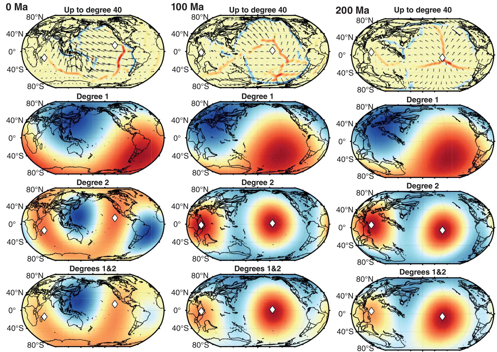
Figure 1.7 Divergence component of plate motions computed for 0, 100, and 200 Ma. In the top row, we show the divergence field up to spherical harmonic degree 40. Red colors indicate positive divergence (spreading) while blue colors indicate convergence. The second row shows only the spherical harmonic degree‐1 component of the divergence field, which represents the net motion of the plates between antipodal centers of long‐wavelength convergence and divergence. The third row shows the spherical harmonic degree‐2 component of the divergence, and the bottom row shows the sum of degrees 1 and 2. The white diamonds in the bottom two rows indicate the locations of the degree‐2 divergence maxima (i.e., centers of degree‐2 spreading).