Magdalena Salazar-Palma - Modern Characterization of Electromagnetic Systems and its Associated Metrology

To illustrate the point, we now perform a rank‐1 approximation for the matrix and we will require

(1.22)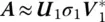

where U 1is a column matrix of size 20×1 and so is V 1. The rank one approximation of Ais seen in Figure 1.2.

The advantage of the SVD is that an error in the reconstruction of the image can be predicted without actually knowing the actual solution. This is accomplished by looking at the second largest singular value. The result is not good and we did not expect it to be. So now if we perform a Rank‐2 reconstruction for the image, it will be given by

(1.23)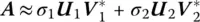

Figure 1.2 Rank‐1 approximation of the image X.

where now two of the right and the left singular values are required. In this case the reank‐2 approximation will be given by Figure 1.3. In this case we have captured the largest two singular values as seen from Table 1.1.

Again as we study how the picture evolves as we take more and more on the singular values and the vectors the accuracy in the reconstruction increases. For example, Figure 1.4provides the rank‐3 reconstruction, Figure 1.5provides the rank‐4 reconstruction, Figure 1.6provides the rank‐5 reconstruction, Figure 1.7provides the rank‐6 reconstruction. It is seen with each higher rank approximation the reconstructed picture resembles the actual one. The error in the approximation decreases as the magnitudes of the neglected singular values become small. This is the greatest advantage of the Singular Value Decomposition over say for example, the Tikhonov regularization as the SVD provides an estimate about the error in the reconstruction even though the actual solution is unknown.

Finally, it is seen that there are seven large singular values and after that they become mostly zeros. Therefore, we should achieve a perfect reconstruction with Rank‐7 which is seen in Figure 1.8and going to rank‐8 which is presented in Figure 1.9, will not make any difference in the quality of the image. This is now illustrated next through the mean squared error between the true solution and the approximate ones.

Figure 1.3 Rank‐2 approximation of the image X.

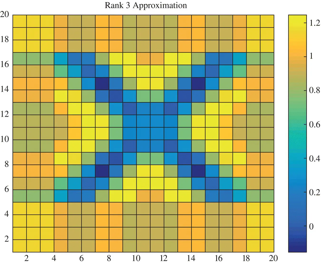
Figure 1.4 Rank‐3 approximation of the image X.

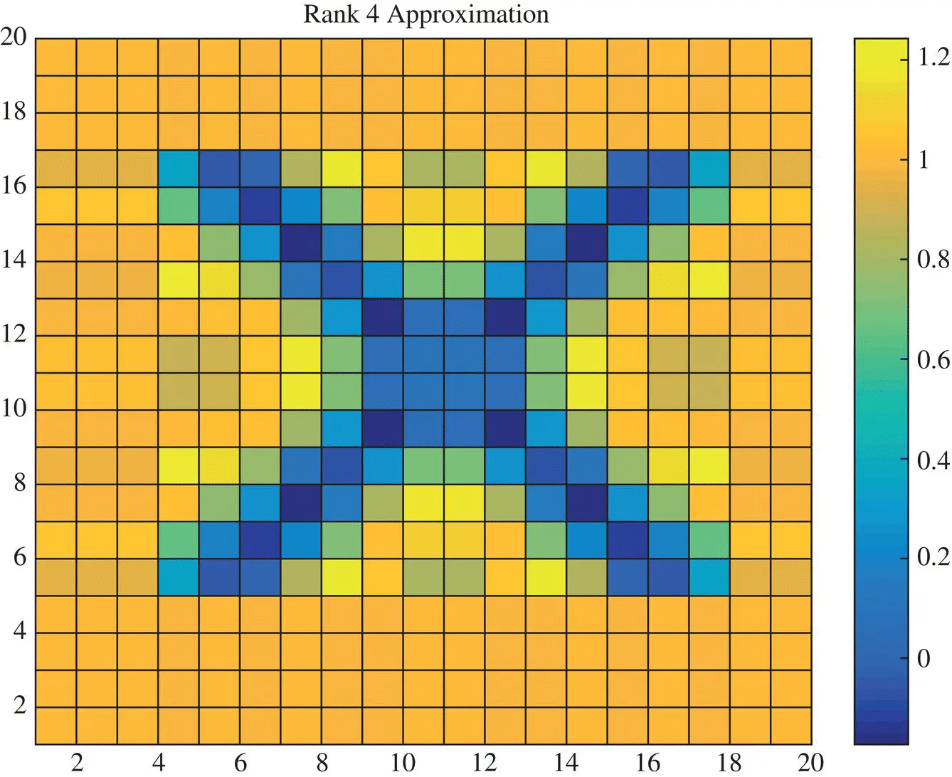
Figure 1.5 Rank‐4 approximation of the image X.

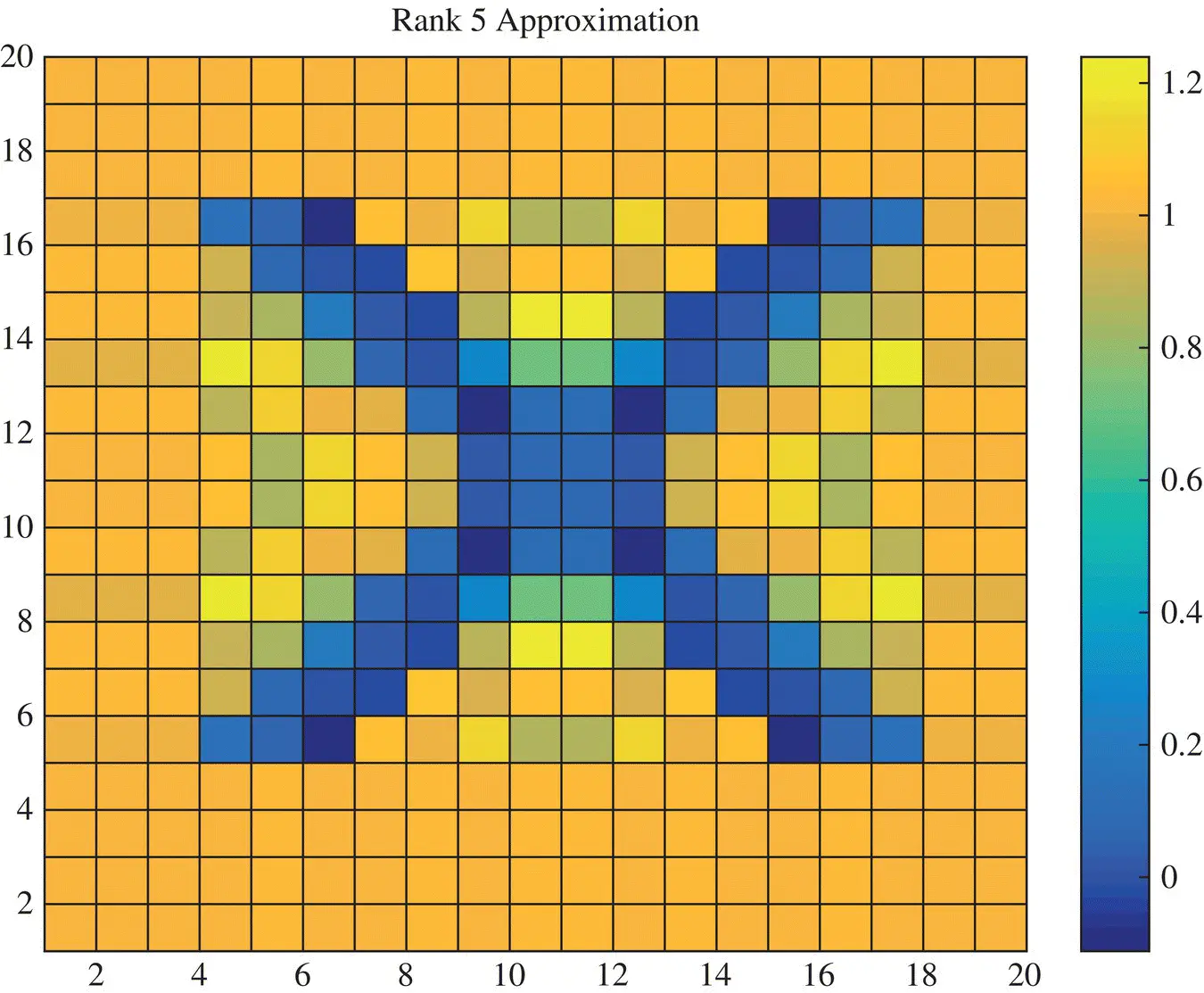
Figure 1.6 Rank‐5 approximation of the image X.

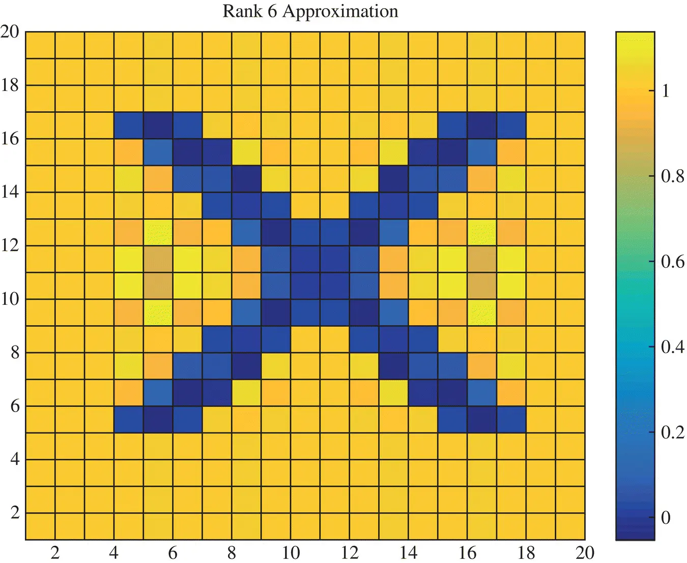
Figure 1.7 Rank‐6 approximation of the image X.

Figure 1.8 Rank‐7 approximation of the image X.

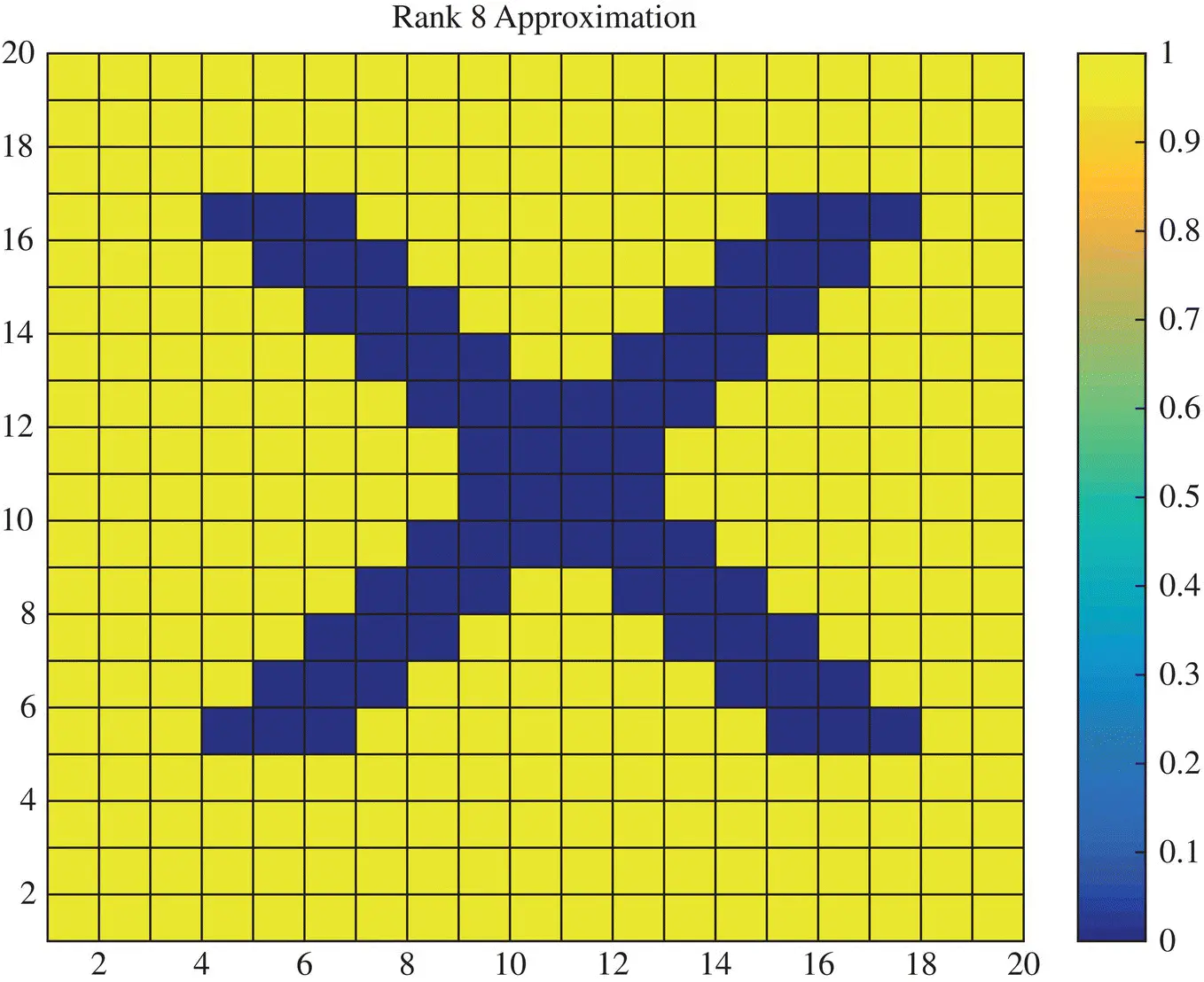
Figure 1.9 Rank‐8 approximation of the image X.

In Figure 1.10, the mean squared error between the actual picture and the approximate ones is presented. It is seen, as expected the error is given by this data

(1.24)

This is a very desirable property for the SVD. Next, the principles of total least squares is presented.

The method of total least squares (TLS) is a linear parameter estimation technique and is used in wide variety of disciplines such as signal processing, general engineering, statistics, physics, and the like. We start out with a set of m measured data points {( x 1 ,y 1),…,( x m ,y m)}, and a set of n linear coefficients ( a 1 ,…,a n) that describe a model, ( x;a ) where m > n [3, 4]. The objective of total least squares is to find the linear coefficients that best approximate the model in the scenario that there is missing data or errors in the measurements. We can describe the approximation by a simple linear expression

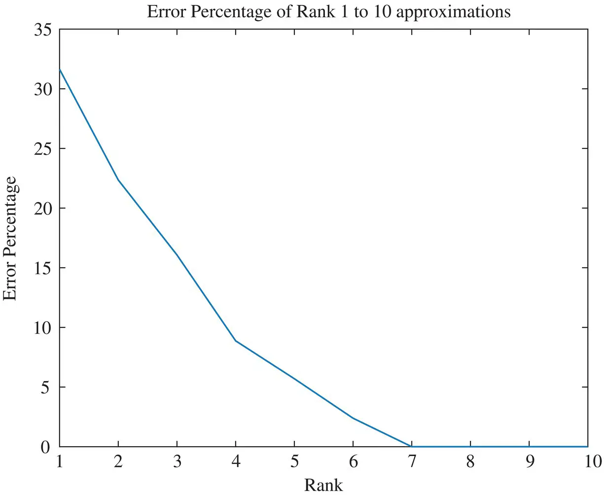
Figure 1.10 Mean squared error of the approximation.

(1.25)

Since m > n , there are more equations than unknowns and therefore (1.25)has an overdetermined set of equations. Typically, an overdetermined system of equation is best solved by the ordinary least squares where the unknown is given by

(1.26)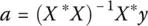

where X ∗represents the complex conjugate transpose of the matrix X . The least squares can take into account if there are some uncertainties like noise in y as it is a least squares fit to it. However, if there is uncertainty in the elements of the matrix X then the ordinary least squares cannot address it. This is where the total Least squares come in. In the total least squares the matrix equation (1.25)is cast into a different form where uncertainty in the elements of both the matrix X and y can be taken into account.

(1.27)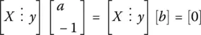

In this form one is solving for the solution to the composite matrix by searching for the eigenvector/singular vector corresponding to the zero eigen/singular value. If the matrix X is rectangular then the eigenvalue concept does not apply and one needs to deal with the singular vectors and the singular values.