Magdalena Salazar-Palma - Modern Characterization of Electromagnetic Systems and its Associated Metrology

In summary, WSS is a less restrictive stationary process and uses a somewhat weaker type of stationarity. It is based on requiring the mean to be a constant in time and the covariance sequence to depend only on the separation in time between the two samples. The final goal in model order reduction of a WSS is to transform the M ‐dimensional vector to a p ‐dimensional vector, where p < M . This transformation is carried out using the Karhunen‐Loeve expansion [2]. The data vector is expanded in terms of q i, the eigenvectors of the correlation matrix [ R ], defined by

(1.4)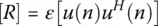

and the superscript H represents the conjugate transpose of u ( n ). Therefore, one obtains

(1.5)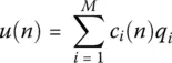

so that

(1.6)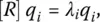

where { λ i} are the eigenvalues of the correlation matrix, { q i} represent the eigenvectors of the matrix R , and { c i( n )} are the coefficients defined by

(1.7)

To obtain a reduced rank approximation of u ( n ), one needs to write

(1.8)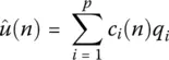

where p < M . The reconstruction error Ξ is then defined as

(1.9)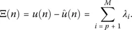

Hence the approximation will be good if the remaining eigenvalues λ p + 1, … λ Mare all very small.

Now to illustrate the implications of a low rank model [2], consider that the data vector u ( n ) is corrupted by the noise v ( n ). Then the data y ( n ) is represented by

(1.10)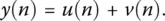

Since the data and the noise are uncorrelated,

(1.11)

where [0] and [Ι] are the null and identity matrices, respectively, and the variance of the noise at each element is σ 2. The mean squared error now in a noisy environment is

(1.12)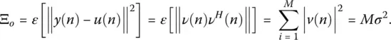

Now to make a low‐rank approximation in a noisy environment, define the approximated data vector by

(1.13)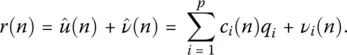

In this case, the reconstruction error for the reduced‐rank model is given by

(1.14)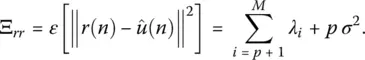

This equation implies that the mean squared error Ξ rrin the low‐rank approximation is smaller than the mean squared error Ξ oto the original data vector without any approximation, if the first term in the summation is small. So low‐rank modelling provides some advantages provided

(1.15)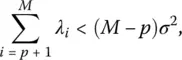

which illustrates the result of a bias‐variance trade off. In particular, it illustrates that using a low‐rank model for representing the data vector u ( n ) incurs a bias through the p terms of the basis vector. Interestingly enough, introducing this bias is done knowingly in return for a reduction in variance, namely the part of the mean squared error due to the additive noise vector v ( n ). This illustrates that the motivation for using a simpler model that may not exactly match the underlying physics responsible for generating the data vector u(n), hence the bias, but the model is less susceptible to noise, hence a reduction in variance [1, 2].

We now use this principle in the interpolation/extrapolation of various system responses. Since the data are from a linear time invariant (LTI) system that has a bounded input and a bounded output and satisfy a second‐order partial differential equation, the associated time‐domain eigenvectors are sums of complex exponentials and in the transformed frequency domain are ratios of two polynomials. As discussed, these eigenvectors form the optimal basis in representing the given data and hence can also be used for interpolation/extrapolation of a given data set. Consequently, we will use either of these two models to fit the data as seems appropriate. To this effect, we present the Matrix Pencil Method (MP) which approximates the data by a sum of complex exponentials and in the transformed domain by the Cauchy Method (CM) which fits the data by a ratio of two rational polynomials. In applying these two techniques it is necessary to be familiar two other topics which are the singular value decomposition and the total least squares which are discussed next.

As has been described in [ https://davetang.org/file/Singular_Value_Decomposition_Tutorial.pdf] “ Singular value decomposition (SVD) can be looked at from three mutually compatible points of view. On the one hand, we can see it as a method for transforming correlated variables into a set of uncorrelated ones that better expose the various relationships among the original data items. At the same time, SVD is a method for identifying and ordering the dimensions along which data points exhibit the most variation. This ties in to the third way of viewing SVD, which is that once we have identified where the most variation is, it's possible to find the best approximation of the original data points using fewer dimensions. Hence, SVD can be seen as a method for data reduction . We shall illustrate this last point with an example later on.

First, we will introduce a critical component in solving a Total Least Squares problem called the Singular Value Decomposition (SVD). The singular value decomposition is one of the most important concepts in linear algebra [2]. To start, we first need to understand what eigenvectors and eigenvalues are as related to a dynamic system. If we multiply a vector xby a matrix [ A], we will get a new vector, Ax. The next equation shows the simple equation relating a matrix [ A] and an eigenvector xto an eigenvalue λ (just a number) and the original x.