Magdalena Salazar-Palma - Modern Characterization of Electromagnetic Systems and its Associated Metrology

Magdalena Salazar Palma

Ming Da Zhu

Heng Chen

In the mathematical field of numerical analysis, model order reduction is the key to processing measured data. This also enables us to interpolate and extrapolate measured data. The philosophy of model order reduction is outlined in this chapter along with the concepts of total least squares and singular value decomposition.

In mathematical physics many problems are characterized by a second order partial differential equation for a function as

(1.1)

and u ( x , y ) is the function to be solved for a given excitation f ( x , y ), where

(1.2)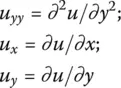

When Β 2− AC < 0 and assuming u xy= u yx, then (1.1)is called an elliptic partial differential equation. These classes of problems arise in the solution of boundary value problems. In this case, the solution u ( x , y ) is known only over a boundary {or equivalently a contour B ( x , y )} and the goal is to continue the given solution u ( x , y ) from the boundary to the entire region of the real plane ℜ( x , y ).

When B 2− AC = 0 we obtain a parabolic partial differential equation for (1.1), which arises in the solution of the diffusion equation or an acoustic propagation in the ocean. Such applications are characterized by the term initial value problems. The solution is given for the initial condition u ( x , y = 0) and the goal is to find the solution u ( x , y ) for all values of x and y .

Finally when Β 2− AC > 0, we obtain a hyperbolic partial differential equation. This type of equation arises from the solution of the wave equation. The characteristic of the wave equation is that if a disturbance is made in the initial data, then not every point of space feels the disturbance at once. The disturbance has a finite propagation speed. This feature makes it distinct from the elliptic and parabolic partial differential equations when a disturbance of the initial data is felt at once by all points in the domain. Even though these equations have significantly different mathematical properties, the solution methodology, just like for every numerical method in solution of an operator equation, is essentially the same, by exploiting the principle of analytic continuation.

The solution u of these equations is made in a straight forward fashion by assuming: it to be of the form

(1.3)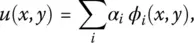

where ϕ i( x , y ) are some known basis functions; and the final solution is to be composed of these functions multiplied by some constants α iwhich are the unknowns to be determined using the specific given boundary conditions. The solution procedure then translates the solution of a functional equation to the solution of a matrix equation, the solution of these unknown constants is much easier to address. The methodology starts by substituting (1.3)into (1.1)and then solving for the unknown coefficients α ifrom the boundary conditions for the problem if the equations are in the differential form or by integrating if it is an integral equation. Then once the unknown coefficients α iare determined, the general solution for the problem can be obtained using (1.3).

A question that is now raised is: what is the optimum way to choose the known basis functions ϕ ias the quality of the final solution depends on the choice of ϕ i? It is well known in the numerical community that the best choices of the basis functions are the eigenfunctions of the operator that characterizes the system. Since in most examples one is dealing with a real life system, then the operators, in general, are linear time invariant (LTI) and have a bounded input and bounded output (BIBO) response resulting in a second‐order differential equation, which is the case for Maxwell’s equations. In the general case, the eigenfunctions of these operators are the complex exponentials, and in the transformed domain, they form a ratio of two rational polynomials. Therefore, our goal is to fit the given data for a LTI system either by a sum of complex exponentials or in the transformed domain approximate it by a ratio of polynomials. Next, it is illustrated how the eigenfunctions are used through a bias‐variance tradeoff in reduced rank modelling [1, 2].

An important problem in statistical processing of waveforms is that of feature selection, which refers to a transformation whereby a data space is transformed into a feature space that, in theory, has exactly the same dimensions as that of the original space [2]. However, in practical problems, it may be desirable and often necessary to design a transformation in such a way that the data vector can be represented by a reduced number of “effective” features and yet retain most of the intrinsic information content of the input data. In other words, the data vector undergoes a dimensionality reduction [1, 2]. Here, the same principle is applied by attempting to fit an infinite‐dimensional space given by (1.3)to a finite‐dimensional space of dimension p .

An important problem in this estimation of the proper rank is very important. First if the rank is underestimated then a unique solution is not possible. If on the other hand the estimated rank is too large the system equations involved in the parameter estimation problem can become very ill‐conditioned, leading to inaccurate or completely erroneous results if straight forward LU‐decomposition is used to solve for the parameters. Since, it is rarely a “crisp” number that evolves from the solution procedure determining the proper rank requires some analysis of the data and its effective noise level. An approach that uses eigenvalue analysis and singular value decomposition for estimating the effective rank of given data is outlined here.

As an example, consider an M ‐dimensional data vector u ( n ) representing a particular realization of a wide‐sense stationary process. (Stationarity refers to time invariance of some, or, all of the statistics of a random process, such as mean, autocorrelation, n th‐order distribution. A random process X ( t ) [or X ( n )] is said to be strict sense stationary (SSS) if all its finite order distributions are time invariant, i.e., the joint cumulative density functions (cdfs), or probability density functions (pdfs), of X ( t 1), X ( t 2), …, X ( t k) and X ( t 1+ τ ), X ( t 2+ τ ), …, X ( t k+ τ ) are the same for all k , all t 1, t 2, …, t k, and all time shifts τ . So for a SSS process, the first‐order distribution is independent of t , and the second‐order distribution — the distribution of any two samples X ( t 1) and X ( t 2) — depends only on τ = t 2− t 1To see this, note that from the definition of stationarity, for any t , the joint distribution of X ( t 1) and X ( t 2) is the same as the joint distribution of X { t –1+ ( t − t 1)} = X ( t ) and X { t 2+ ( t − t 1)} = X { t + ( t 2– t )}. An independent and identically distributed (IID) random processes are SSS. A random walk and Poisson processes are not SSS. The Gauss‐Markov process (as we defined it) is not SSS. However, if we set X 1to the steady state distribution of X n, it becomes SSS. A random process X ( t ) is said to be wide‐sense stationary (WSS) if its mean, i.e., ε ( X ( t )) = μ , is independent of t , and its autocorrelation functions RX ( t 1, t 2) is a function only of the time difference t 2− t 1and are time invariant. Also ε [ X ( t ) 2] < ∞ (technical condition) is necessary, where ε represents the expected value in a statistical sense. Since RX ( t 1, t 2) = RX ( t 2, t 1), for any wide sense stationary process X ( t ), RX ( t 1, t 2) is a function only of | t 2– t 1|. Clearly a SSS implies a WSS. The converse is not necessarily true. The necessary and sufficient conditions for a function to be an autocorrelation function for a WSS process is that it be real, even, and nonnegative definite By nonnegative definite we mean that for any n , any t 1, t 2, …, t nand any real vector a = ( a 1, …, a n), and X ( n ); a i a j R ( t i− t j) ≥ 0. The power spectral density (psd) SX ( f ) of a WSS random process X ( t ) is the Fourier transform of RX ( τ ), i.e., SX ( f ) = ℑ { RX ( τ )} = 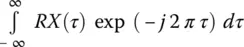. For a discrete time process X n, the power spectral density is the discrete‐time Fourier transform (DTFT) of the sequence RX ( n ): SX ( f ) = 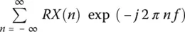. Therefore RX ( τ ) (or RX ( n )) can be recovered from SX ( f ) by taking the inverse Fourier transform or inverse DTFT.