Yong Chen - Industrial Data Analytics for Diagnosis and Prognosis

(3.26)

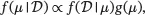
where ∝ stands for “is proportional to”. Note the denominator p ( D ) in the right-hand side of ( 3.25) is a constant which does not depend on the parameter μ. It plays the normalization role to ensure the left-hand side is a valid probability density function and integrates to one. Taking the integral of the right-hand side of ( 3.25) with respect to μand setting it to be equal to one, it is easy to see that

A point estimate of μcan be obtained by maximizing the posterior distribution. This method is called the maximum a posteriori (MAP) estimate. The MAP estimate of μcan be written as

(3.27)

From ( 3.27), it can be seen that the MAP estimate is closely related to MLE. Without the prior g ( μ), the MAP is the same as the MLE. So if the prior follows a uniform distribution, the MAP and MLE will be equivalent. Following this argument, if the prior distribution has a flat shape, we expect that the MAP and MLE are similar.

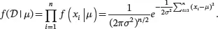
We first consider a simple case where the data follow a univariate normal distribution with unknown mean μ and known variance σ 2. The likelihood function based on a random sample of independent observations D = { x 1, x 2,…, xn } is given by

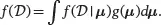
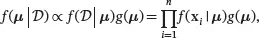
Based on ( 3.26), we have

where g ( μ ) is the probability density function of the prior distribution. We choose a normal distribution N ( μ 0, σ 0 2) as the prior for μ . This prior is a conjugate prior because the resulting posterior distribution will also be normal. By completing the square in the exponent of the likelihood and prior, the posterior distribution can be obtained as

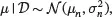
where

(3.28)

(3.29)

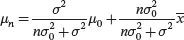
The posterior mean given in ( 3.28) can be understood as a weighted average of the prior mean μ 0and the sample mean x̄ , which is the MLE of μ . When the sample size n is very large, the weight for x̄ is close to one and the weight for μ 0is close to 0, and the posterior mean is very close to the MLE, or the sample mean. On the other hand, when n is very small, the posterior mean is very close the prior mean μ 0. Similarly, if the prior variance σ 0 2is very large, the prior distribution has a flat shape and the posterior mean is close to the MLE. Note that because the mode of a normal distribution is equal to the mean, the MAP of μ is exactly μn . Consequently, when n is very large, or when the prior is flat, the MAP is close to the MLE.

Equation ( 3.29) shows the relationship between the posterior variance and the prior variance. It is easier to understand the relationship if we consider the inverse of the variance, which is called the precision . A high (low) precision corresponds to a low (high) variance. Equation ( 3.29) basically says that the posterior precision is equal to the prior precision with an added precision contribution proportional to n . Each observation adds a contribution of , the precision of xn , to the posterior precision. When n is very large, the posterior precision becomes very high, or equivalently the posterior variance becomes very small. On the other hand, when n is very small, the posterior precision and variance will be very close to the prior precision and variance. Specifically, when n = 0, the posterior distribution is the same as the prior distribution. We illustrate the posterior distribution of the mean with known variance under various sample sizes in Figure 3.3, where the data are generated from N (2, 1) and the prior distribution of the mean is N (0, 1). It is clear from Figure 3.3 that with sample size n getting larger, the posterior distribution of the mean becomes more and more concentrated at the true mean.

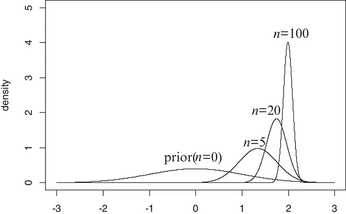
Figure 3.3 Posterior distribution of the mean with various sample sizes

When the data follow a p -dimensional multivariate normal distribution with unknown mean μand known covariance matrix Σ, the posterior distribution based on a random sample of independent observations D = { x 1, x 2,…, x n} is given by

where g ( μ) is the density of the conjugate prior distribution Np ( μ 0, Σ 0). Similar to the univariate case, the posterior distribution of μcan be obtained as

where

(3.30)

(3.31)

where x̄is the sample mean of the data, which is the MLE of μ. It is easy to see the similarity between the results for the univariate data in ( 3.28) and ( 3.29) and the results for the multivariate data in ( 3.30) and ( 3.31). The MAP of μis exactly μ n . Similar to the univariate case, when n is large, or when the prior distribution is flat, the MAP is close to the MLE.