Magnetic Nanoparticles in Human Health and Medicine

To conclude, if in the case of bulk magnetic material, the saturation magnetization is a well‐defined value, being a material parameter, characteristic of the substance type, in the case of nanoparticles it is generally smaller, and decreases with the decrease in diameter to nanometers size. This is a very important aspect that must be taken into account in biomedical applications. Thus, in order not to introduce errors in the application of magnetic nanoparticles, it is recommended, before conducting any experiment, to determine/measure the saturation magnetization of the nanoparticles, and also the variation of saturation magnetization with temperature, if there is such a dependency in the targeted application.

Experimentally, it was found that in the case of ferro‐ or ferrimagnetic crystalline materials, there is a dependence of the magnetization of the single crystal on the crystallographic directions. The dependence of the magnetization of the crystalline magnetic material on the crystallographic axes determines the magnetocrystalline anisotropy (Kneller 1962; Caizer 2004a, 2019). Thus, the magnetization curves that are obtained in the same external magnetic field depend on the direction in which the crystalline material is magnetized. This type of magnetic anisotropy is characteristic of all bulk single crystalline (ferro‐ or ferromagnetic) magnetic materials (Fe, Co, Ni, Cd, their alloys, Fe oxides [Fe 3O 4, γ‐Fe 2O 3], etc.).

For example, in the case of the Ni bulk single crystal ferromagnetic material, which crystallizes in the cube system with centered volume (vcc), the magnetization curves have the shape shown in Figure 1.8(Baberschke 2001). Thus, the magnetization is made easiest following the crystallographic direction [1,1,1], which represents the large diagonal of the cube, and its magnetization is made the hardest following the crystallographic direction [1,0,0], which is the edge of the cube. The direction [1,1,1] in this case is called the direction or axis of easy magnetization (e.m.a.), and the direction [1,0,0] is called the axis of hard magnetization (h.m.a).

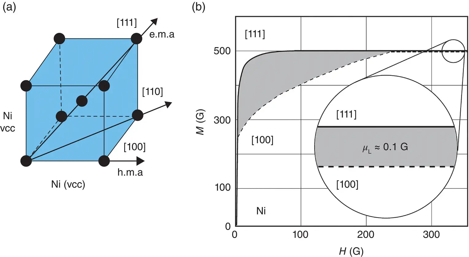
Figure 1.8 (a) The crystallographic systems for Ni‐single crystal.

Source: Caizer (2016). Reprinted by permission from Springer Nature;

(b) Room temperature magnetization curves for Ni along the easy ([111]) and hard ([100]) direction.

Source: Based on Wijn (1986).

In the case of bulk ferromagnetic monocrystalline material with cubic symmetry, the energy of magnetocrystalline anisotropy can be determined with the following formula:

(1.15)

written as a series development of powers using the model proposed by Beker, Doring, Akulov, Mason (Kneller 1962; Herpin 1968), based on the symmetry properties of the crystal. In general, it was found that it is sufficient to use only the first two terms of development, in K 1and K 2. In Eq. (1.15), K 1and K 2are the magnetocystalline anisotopy constants, and α 1, α 2and α 3are the cosine directors of the vector of spontaneous magnetization ( M s) in relation to the main crystallographic axes of the cube. In some cases, even the first term of development is sufficient. For example, in the case of the ferromagnetic Fe single crystal, K 1= 4.8 × 10 4J m −3and K 2= 5 × 10 3J m −3were found, where K 1is in this case with approximately one order of magnitude larger than K 2.

In the case of uniaxial, hexagonal symmetry, as in the case of the ferromagnetic Co monocrystalline ( Figure 1.9), the magnetocrystalline anisotropy energy is expressed as a function of the angle fi between the spontaneous magnetization vector M sand the main axis of symmetry:

(1.16)

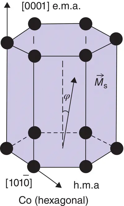
Figure 1.9 The crystallographic systems for Co‐single crystal.

Source: Caizer (2016). Reprinted by permission from Springer Nature.

Also, in this case, the first two terms are used (in K 1and K 2) in the energy expression of uniaxial magnetocrystalline anisotropy.

In this case, the main axis of symmetry is the easy magnetization axis (e.m.a), and the direction perpendicular to it is the hard magnetization axis (h.m.a).

In the case of bulk magnetic material, there is another important form of magnetic anisotropy, which should not be neglected as it can become dominant in some cases. This is the anisotropy of the shape (Kneller 1962; Caizer 2004a), which shows that the magnetization of a sample depends on its shape.

As a general case, approximating the shape of the sample by the ellipsoid of revolution: a > b = c , where a , b , and c are the semiaxes of the ellipsoid ( Figure 1.10), the anisotropy energy due to the shape of the sample is expressed by the following formula:

(1.17)

where N aand N bare the demagnetization factors along the a and b directions of the ellipsoid, and θ is the angle that the spontaneous magnetization vector M smakes with the main axis ( a ) of the ellipsoid.

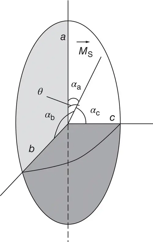
Figure 1.10 The crystal approximated by an ellipsoid (general case).

Source: Caizer (2019). Reprinted by permission of Taylor & Francis Ltd.

When the magnetization of the ellipsoid in the external magnetic field is done along the direction of the a ‐axis, the shape anisotropy energy is minimum (or zero). In contrast, when magnetization is done along a direction perpendicular to the a ‐axis (e.g. the b , c , or other directions), the shape anisotropy energy is maximum. In the latter case, taking into account the Eqs (1.17)and (1.16), the shape anisotropy constant can be expressed by the following formula:

(1.18)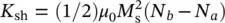

in the approximation of the first order.

When the magnetic material is reduced to the nanoscale, these forms of magnetic anisotropy remain valid. In addition, in the case of magnetic nanoparticles, the shape anisotropy becomes very important, reaching in some cases even larger, or much larger than the magnetocrystalline anisotropy. Thus, the neglect of this first aspect leads to important errors from a magnetic point of view, incompatible with the physical reality. For example, if the nanoparticle is spherical in shape ( Figure 1.5), the semiaxes a , b , c become equal ( Figure 1.10), and equal to the radius of the sphere. According to Eqs. the shape anisotropy constant in this case is zero, as is the energy. So there is no shape anisotropy in the case of spherical nanoparticles. In contrast, in the case of elongated nanoparticles, when a ≫ b = c , and when they are soft magnetic (magnetocrystalline anisotropy is reduced), the shape anisotropy exceeds the magnetocrystalline anisotropy, or even becomes dominant. This is an important aspect in the case of magnetic nanoparticles that must be taken into account not only in practical applications, including biomedical ones, but also in theoretical calculations and models/experiments.