Saeid Sanei - EEG Signal Processing and Machine Learning

(4.123)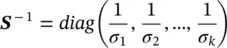

In order to see the application of the SVD in solving the LS problem consider the error vector edefined as:

(4.124)

where dis the desired signal vector and Ahis the estimate . To find hwe replace Awith its SVD in the above equation ( Eq. 4.124) and find h,which thereby minimizes the squared Euclidean norm of the error vector, ‖ e 2‖. By using the SVD we obtain:

(4.125)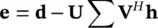

or equivalently

(4.126)

Since Uis a unitary matrix, ‖ e 2‖ = ‖ U H e‖ 2. Hence, the vector hthat minimizes ‖ e 2‖ also minimizes ‖ U H e‖ 2. Finally, the unique solution as an optimum h(coefficient vector) may be expressed as [43]:

(4.127)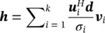

where k is the rank of A. Alternatively, as the optimum least‐squares coefficient vector:

(4.128)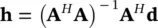

Performing PCA is equivalent to performing an SVD on the covariance matrix. PCA uses the same concept as SVD and orthogonalization to decompose the data into its constituent uncorrelated orthogonal components such that the autocorrelation matrix is diagonalized. Each eigenvector represents a principal component and the individual eigenvalues are numerically related to the variance they capture in the direction of the principal components. In this case the mean squared error (MSE) is simply the sum of the N‐K eigenvalues, i.e.:

(4.129)

PCA is widely used in data decomposition, classification, filtering, and whitening. In filtering applications, the signal and noise subspaces are separated and the data are reconstructed from only the eigenvalues and eigenvectors of the actual signals. PCA is also used for BSS of correlated mixtures if the original sources can be considered statistically uncorrelated.

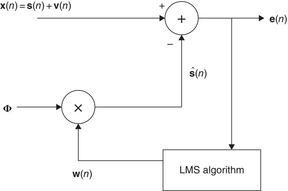
Figure 4.13 Adaptive estimation of the weight vector w( n ).

The PCA problem is then summarized as how to find the weights win order to minimize the error given the observations only. The LMS algorithm is used here to iteratively minimize the MSE as:

(4.130)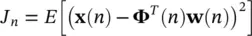

The update rule for the weights is then:

(4.131)

where the error signal e( n ) = x( n ) − Φ T( n ) w( n ), x( n ) is the noisy input and n is the iteration index. The step size μ may be selected empirically or adaptively. These weights are then used to reconstruct the sources from the set of orthogonal basis functions. Figure 4.13shows the overall system for adaptive estimation of the weight vector wusing the LMS algorithm.

In this chapter some basic signal processing tools and algorithms applicable to EEG signals have been reviewed. These fundamental techniques can be applied to reveal the inherent structure and the major characteristics of the signals based on which the state of the brain can be determined. TF‐domain analysis is indeed a good EEG descriptive for both normal and abnormal cases. The change in entropy Conversely, may describe the transitions between preictal to ictal states for epileptic patients. These concepts will be exploited in the following chapters of this book.

1 1 Lebedev, M.A. and Nicolelis, M.A. (2006). Brain‐machine interfaces: past, present and future. Trends in Neurosciences 29: 536–546.

2 2 Lopes Da Silva, F. (2004). Functional localization of brain sources using EEG and/or MEG data: volume conductor and source models. Journal of Magnetic Resonance Imaging 22 (10): 1533–1538.

3 3 Durka, P.J., Dobieslaw, I., and Blinowska, K.J. (2001). Stochastic time–frequency dictionaries for matching pursuit. IEEE Transactions on Signal Processing 49 (3).

4 4 Spyrou, L., Lopez, D.M., Alarcon, G. et al. (2016). Detection of intracranial signatures of interictal epileptiform discharges from concurrent scalp EEG. International Journal of Neural Systems 26 (4): 1650016.

5 5 Spyrou, L., Kouchaki, S., and Sanei, S. (2016). Multiview classification and dimensionality reduction of EEG data through tensor factorisation. Journal of Signal Processing Systems 90: 273–284.

6 6 Spyrou, L. and Sanei, S. (2016). Coupled dictionary learning for multimodal data: an application to concurrent intracranial and scalp EEG. 2016 IEEE International Conference on Acoustics, Speech and Signal Processing (ICASSP), 2349–2353. Shanghai, China.

7 7 Antoniades, A., Spyrou, L., Martin‐Lopez, D. et al. (2018). Deep neural architectures for mapping scalp to intracranial EEG. International Journal of Neural Systems 28 (8): 1850009. https://doi.org/10.1142/S0129065718500090.

8 8 Antoniades, A., Spyrou, L., Martin‐Lopez, D. et al. (2017). Detection of interictal discharges using convolutional neural networks from multichannel intracranial EEG. IEEE Transactions on Neural Systems and Rehabilitation Engineering 25 (12): 2285–2294.

9 9 Strang, G. (1998). Linear Algebra and its Applications, 3e. Thomson Learning.

10 10 McCann, H., Pisano, G., and Beltrachini, L. (2019). Variation in reported human head tissue electrical conductivity values. Brain Topography 32: 825–858.

11 11 Hyvarinen, A., Kahunen, J., and Oja, E. (2001). Independent Component Analysis. Wiley.

12 12 Cover, T.M. and Thomas, J.A. (2001). Elements of Information Theory. Wiley.

13 13 Azami, H., Arnold, S.E., Sanei, S. et al. (2019). Multiscale fluctuation‐based dispersion entropy and its applications to neurological diseases. IEEE Access 7 (1): 68718–68733, ISSN: 2169‐3536. https://doi.org/10.1109/ACCESS.2019.2918560.