Saeid Sanei - EEG Signal Processing and Machine Learning

(4.61)

where ω lis the nearest frequency to the original point ω ( a , b ), ∆ ω is the width of the frequency bins ,∆ ω = ω l− ω l − 1, and (∆ a ) k= a k− a k − 1. T f( ω l, b ) represents the synchro‐squeezed transform at the centres ω lof consecutive frequency bins. For each fixed time point b , the reassigned frequencies should be estimated for all scales using Eq. (4.103). For each desired IF of ω l, T f( ω l, b ) is calculated using summation of all W ( a k, b ) considering that the distance between the reassigned frequency ω ( a k, b ) and ω lmust be within the specified frequency bin width (∆ ω ). It has been shown that the original signal can be reconstructed after the synchro‐squeezing process [23].

The ambiguity function for a continuous time signal is defined as:

(4.62)

This function has its maximum value at the origin as

(4.63)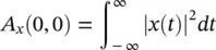

As an example, if we consider a continuous time signal consisting of two modulated signals with different carrier frequencies such as

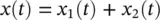
(4.64)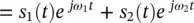

The ambiguity function A x( τ,ν ) will be in the form of:

(4.65)

This concept is very important in separation of signals using the TF domain. This will be addressed in the context of blind source separation (BSS) later in this chapter. Figure 4.8demonstrates this concept.

The Wigner–Ville frequency distribution of a signal x ( t ) is then defined as the two‐dimensional Fourier transform of the ambiguity function:

(4.66)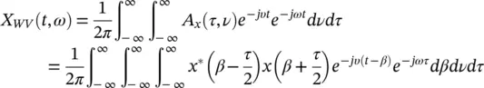

which changes to the dual form of the ambiguity function as:

(4.67)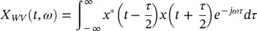

A quadratic form for the TF representation with the Wigner–Ville distribution can also be obtained using the signal in the frequency domain as:

(4.68)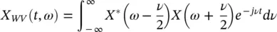

The Wigner–Ville distribution is real and has very good resolution in both the time‐ and frequency‐domains. Also it has time and frequency support properties, i.e. if x ( t ) = 0 for | t | > t 0, then X WV( t , ω ) = 0 for | t | > t 0, and if X ( ω ) = 0 for | ω | > ω 0, then X WV( t , ω ) = 0 for | ω | > ω 0. It has also both time‐marginal and frequency‐marginal conditions of the form:

(4.69)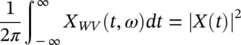

and

(4.70)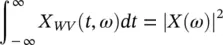

If x ( t ) is the sum of two signals x 1( t ) and x 2( t ), i.e. x ( t ) = x 1( t ) + x 2( t ), the Wigner–Ville distribution of x ( t ) with respect to the distributions of x 1( t ) and x 2( t ) will be:

(4.71)

where Re{.} denotes the real part of a complex value and

(4.72)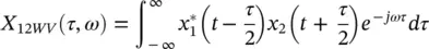

It is seen that the distribution is related to the spectra of both auto‐ and cross‐correlations. A pseudo‐Wigner–Ville distribution (PWVD) is defined by applying a window function, w ( τ ), centred at τ = 0 to the time‐based correlations, i.e.:

(4.73)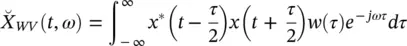

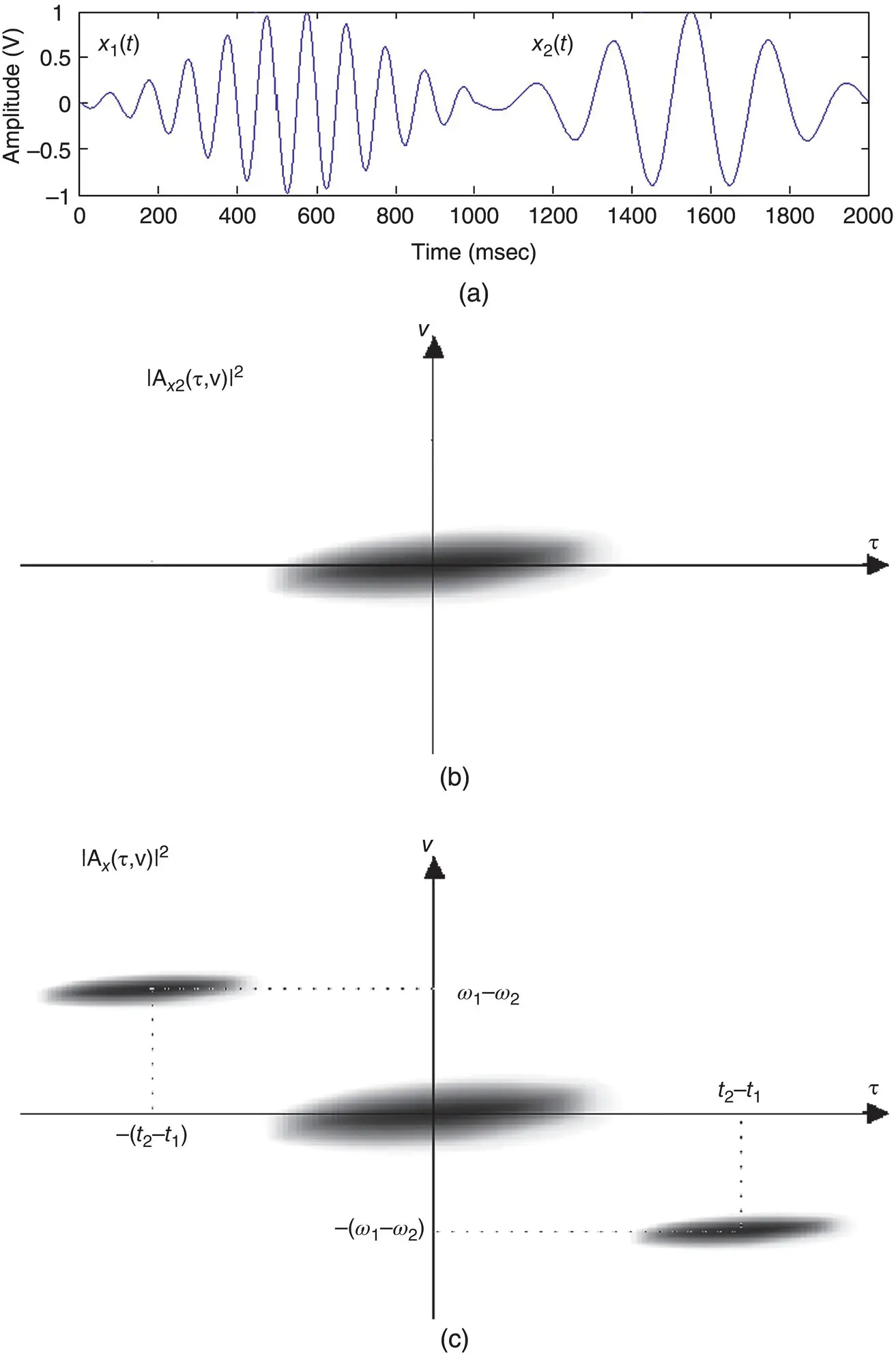
Figure 4.8 (a) A segment of a signal consisting of two modulated components, (b) ambiguity function for x 1( t ) only, and (c) the ambiguity function for x ( t ) = x 1( t ) + x 2( t ).

In order to suppress the undesired cross‐terms the two‐dimensional Wigner–Ville (WV) distribution may be convolved with a TF‐domain window. The window is a two‐dimensional lowpass filter, which satisfies the time and frequency‐marginal (uncertainty) conditions, as described earlier. This can be performed as:

(4.74)

where

(4.75)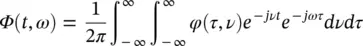

and φ ( τ , ν ) is often selected from a set of well known waveforms called Cohen's class . The most popular member of the Cohen's class of functions is the bell‐shaped function defined as: