Saeid Sanei - EEG Signal Processing and Machine Learning

(4.20)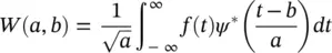

where (.) *denotes the complex conjugate, is the analyzing wavelet, a (>0) is the scale parameter (inversely proportional to frequency) and b is the position parameter. The transform is linear and is invariant under translations and dilations, i.e.:

(4.21)

and

(4.22)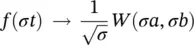

The last property makes the WT very suitable for analyzing hierarchical structures. It is similar to a mathematical microscope with properties that do not depend on the magnification. Consider a function W ( a , b ) which is the WT of a given function f ( t ). It has been shown [18, 19] that f ( t ) can be recovered according to:

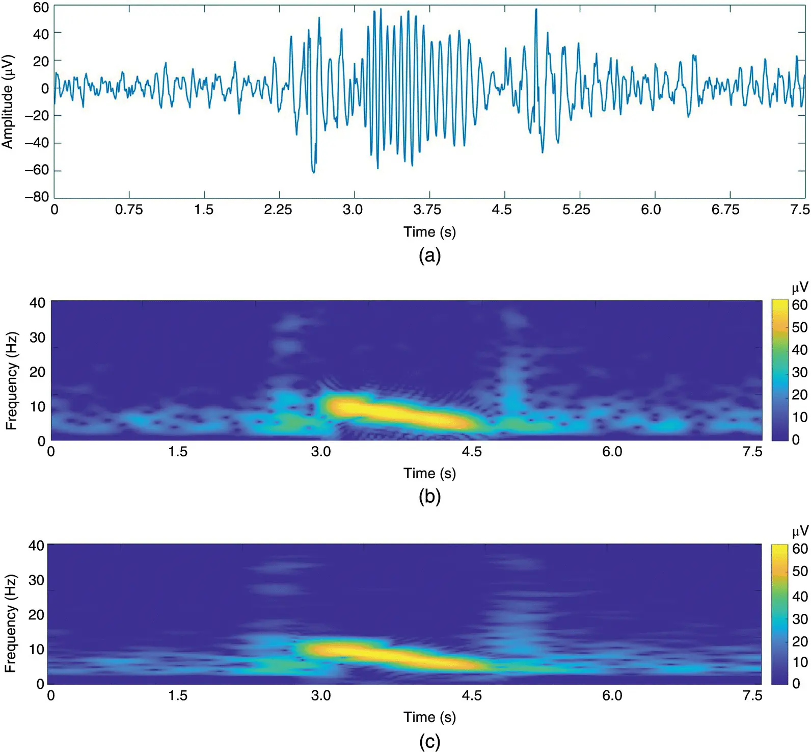
Figure 4.4 TF representation of an epileptic waveform in (a) for different time resolutions using the Hanning window of (b) 1 ms, and (c) 2 ms duration.

(4.23)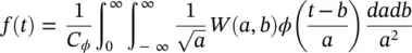

where

(4.24)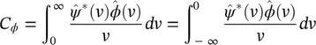

Although often it is considered that ψ ( t ) = ϕ ( t ), other alternatives for ϕ ( t ) may enhance certain features for some specific applications [20]. The reconstruction of f ( t ) is subject to having C ϕdefined (admissibility condition). The case ψ ( t ) = ϕ ( t ) implies , i.e. the mean of the wavelet function is zero.

Different waveforms/wavelets/kernels have been defined for the continuous WTs. The most popular ones are given below.

Morlet's wavelet is a complex waveform defined as:

(4.25)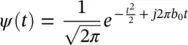

This wavelet may be decomposed into its constituent real and imaginary parts as:

(4.26)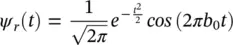

(4.27)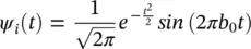

where b 0is a constant, and it is considered that b 0> 0 to satisfy the admissibility condition. Figure 4.5shows respectively the real and imaginary parts.

The Mexican hat defined by Murenzi [17] is:

(4.28)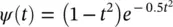

which is the second derivative of a Gaussian waveform (see Figure 4.6).

In order to process digital signals a discrete approximation of the wavelet coefficients is required. The discrete wavelet transform (DWT) can be derived in accordance with the sampling theorem if we process a frequency band‐limited signal.

The continuous form of the WT may be discretized with some simple considerations on the modification of the wavelet pattern by dilation. Since generally the wavelet function is not band limited, it is necessary to suppress the values outside the frequency components above half the sampling frequency to avoid aliasing (overlapping in frequency) effects.

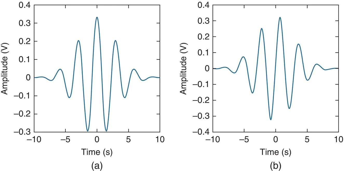
Figure 4.5 Morlet's wavelet: real and imaginary parts shown respectively in (a) and (b).

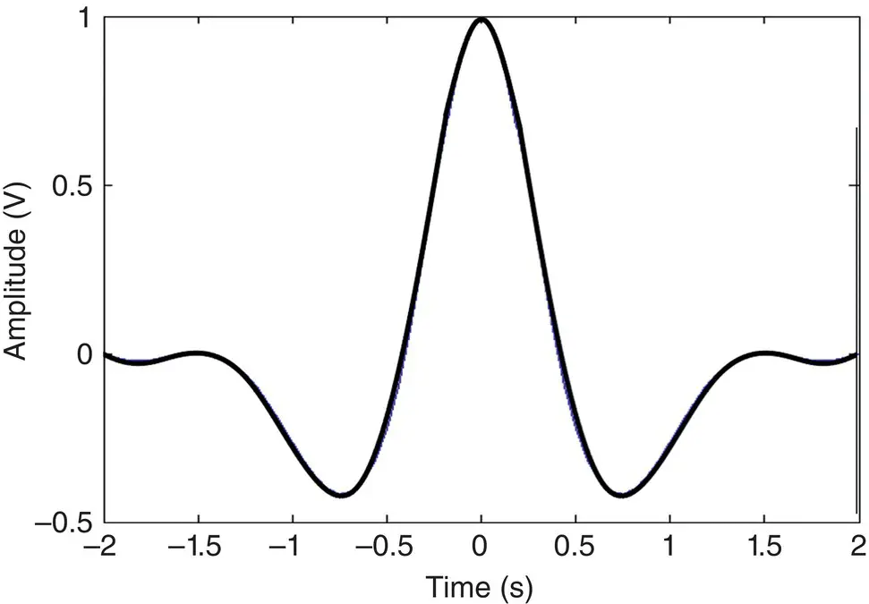
Figure 4.6 Mexican hat wavelet.

A Fourier space may be used to compute the transform scale‐by‐scale. The number of elements for a scale can be reduced if the frequency bandwidth is also reduced. This requires a band‐limited wavelet. The decomposition proposed by Littlewood and Paley [21] provides a very nice illustration of the reduction of elements scale‐by‐scale. This decomposition is based on an iterative dichotomy of the frequency band. The associated wavelet is well localized in Fourier space where it allows a reasonable analysis to be made although not in the original space. The search for a discrete transform, which is well localized in both spaces leads to multiresolution analysis.

Multiresolution analysis results from the embedded subsets generated by the interpolations (or down‐sampling and filtering) of the signal at different scales. A function f ( t ) is projected at each step j onto the subset V j. This projection is defined by the scalar product c j( k ) of f ( t ) with the scaling function φ ( t ), which is dilated and translated:

(4.29)

where 〈·, ·〉 denotes an inner product and φ ( t ) has the property:

(4.30)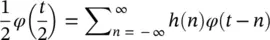

where the right side is convolution of h and ϕ . By taking the Fourier transform of both sides:

(4.31)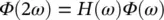

where and are the Fourier transforms of h ( t ) and ϕ ( t ) respectively. For a discrete frequency space (i.e. using the DFT) the above equation ( Eq. 4.31) permits the computation of the wavelet coefficient C j + 1( k ) from C j( k ) directly. If we start from C 0( k ) we compute all C j( k ), with j > 0, without directly computing any other scalar product: