Saeid Sanei - EEG Signal Processing and Machine Learning

It is clear that the KL distance is generally asymmetric, therefore by changing the position of p 1and p 2in this Eq. (4.6)the KL distance changes. The minimum of the KL distance occurs when p 1( z ) = p 2( z ).

Often it is necessary to label the EEG signals into the segments of similar characteristics particularly meaningful to clinicians and for the assessment by neurophysiologists. Within each segment, the signals are considered statistically stationary usually with similar time and frequency statistics. As an example, an EEG recorded from an epileptic patient may be divided into three segments of preictal, ictal, and postictal segments. Each may have a different duration. Figure 4.1represents an EEG sequence including all the above segments.

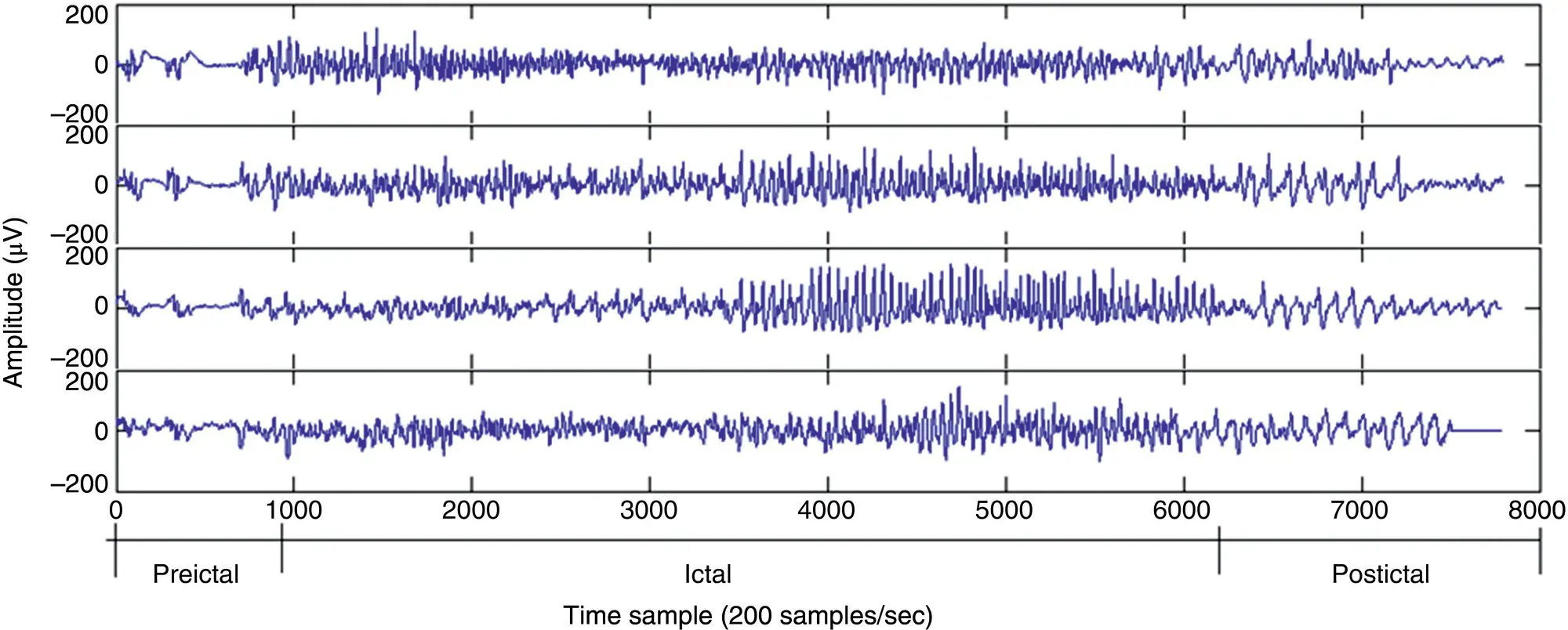
Figure 4.1 An EEG set of tonic–clonic seizure signals including three segments of preictal, ictal, and postictal behaviour.

In segmentation of EEGs time or frequency properties of the signals may be exploited. This eventually leads to a dissimilarity measurement denoted as d ( m ) between the adjacent EEG frames where m is an integer value indexing the frame and the difference is calculated between the m and ( m − 1)th (consecutive) signal frames. The boundary of the two different segments is then defined as the boundary between the m and ( m − 1)th frames provided d ( m ) > η T, and η Tis an empirical threshold level. An efficient segmentation is possible by highlighting and effectively exploiting the diagnostic information within the signals with the help of expert clinicians. However, access to such experts is not always possible and therefore, there are needs for algorithmic methods.

A number of different dissimilarity measures may be defined based on the fundamentals of signal processing. One criterion is based on the autocorrelations for segment m defined as:

(4.7)

The autocorrelation function of the m th length N frame for an assumed time interval n, n + 1, …, n + ( N − 1), can be approximated as:

(4.8)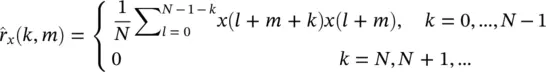

Then the criterion is set to:

(4.9)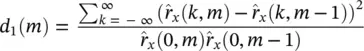

A second criterion can be based on higher‐order statistics. The signals with more uniform distributions such as normal brain rhythms have a low kurtosis, whereas seizure signals or ERP signals often have high kurtosis values. Kurtosis is defined as the fourth‐order cumulant at zero time lags and related to the second‐order and fourth‐order moments as given in Eqs. (4.1)– (4.3). A second level discriminant d 2( m ) is then defined as:

(4.10)

where m refers to the mth frame of the EEG signal x ( n ). A third criterion is defined from the spectral error measure of the periodogram. A periodogram of the m th frame is obtained by Fourier transforming of the correlation function of the EEG signal:

(4.11)

where is the autocorrelation function for the m th frame as defined above. The criterion is then defined based on the normalized periodogram as:

(4.12)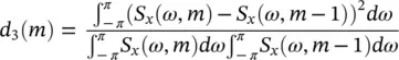

The test window sample autocorrelation for the measurement of both d 1( m ) and d 3( m ) can be updated through the following recursive equation ( Eq. 4.13) over the test windows of size N :

(4.13)

and thereby computational complexity can be reduced in practise. A fourth criterion corresponds to the error energy in autoregressive (AR) ‐based modelling of the signals. The prediction error in the AR model of the m th frame is simply defined as:

(4.14)

where p is the prediction order and a k( m ), k = 1, 2, …, p, are the prediction coefficients. For certain p the coefficients can be found directly (for example by using Durbin's method) in such a way to minimize the error (residual) between the actual and predicted signal energy. In this approach it is assumed that the frames of length N overlap by one sample. The prediction coefficients estimated for the ( m − 1)th frame are then used to predict the first sample in the m th frame, which we denote it as . If this error is small, it is likely that the statistics of the m th frame are similar to those of the ( m − 1)th frame. Conversely, a large value is likely to indicate a change. An indicator for the fourth criterion can then be the differentiation of this signal (difference of digital signal) with respect to time, which gives a peak at the segment boundary, i.e.:

(4.15)

where ∇ n(.) denotes the gradient with respect to n , approximated by a first‐order difference operation. Figure 4.2shows the residual and the gradient defined in Eq. (4.15), wherein the prediction order has been selected as 12.

Finally, a fifth criterion d 5( m ) may be defined by using the AR‐based spectrum of the signals in the same way as short‐time Fourier transform (STFT) for d 3( m ). The above AR model is a univariate model, i.e. it models a single‐channel EEG. A similar criterion may be defined when multichannel EEGs are considered [14]. In such cases a multivariate AR (MVAR) model is analyzed. The MVAR can also be used for characterization and quantification of the signal propagation within the brain and is discussed in Chapter 8of this book.