Saeid Sanei - EEG Signal Processing and Machine Learning

Adaptive noise cancellers used in communications, signal processing, and biomedical signal analysis can also be used for removing noise and artefacts from the EEG signals. An effective adaptive noise canceller however requires a reference signal. Figure 4.11shows a general block diagram of an adaptive filter for noise cancellation. The reference signal carries significant information about the noise or artefact and its statistical properties. For example, in the removal of eye‐blinking artefacts (discussed in Chapter 16) a signature of the eye‐blink signal can be captured from the FP1 and FP2 EEG electrodes. In detection of the ERP signals, as another example, the reference signal can be obtained by averaging a number of ERP segments. There are many other examples such as ECG cancellation from EEGs and the removal of fMRI scanner artefacts from EEG‐fMRI simultaneous recordings where the reference signals can be provided.

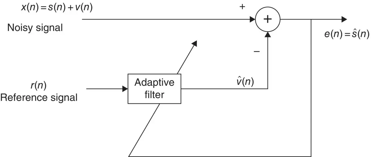
Figure 4.11 An adaptive noise canceller.

Adaptive Wiener filters are probably the most fundamental type of adaptive filters. In Figure 4.11the optimal weights for the filter, w( n ), are calculated such that is the best estimate of the actual signal s( n ) in the mean square sense. The Wiener filter minimizes the mean square value of the error defined as:

(4.91)

where wis the Wiener filter coefficient vector. Using the orthogonality principle [39] the final form of the mean squared error will be:

(4.92)

where E (.) represents statistical expectation:

(4.93)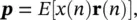

and

(4.94)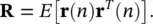

By taking the gradient with respect to wand equating it to zero we have:

(4.95)

As Rand pare usually unknown the above minimization is performed iteratively by substituting time averages for statistical averages. The adaptive filter in this case, decorrelates the output signals. The general update equation is in the form of:

(4.96)

where n is the iteration number which typically corresponds to discrete‐time index. Δ w( n ) has to be computed such that E [ e( n )] 2reaches to a reasonable minimum. The simplest and most common way of calculating Δ w( n ) is by using gradient descent or steepest descent algorithm [39]. In both cases, a criterion is defined as a function of the squared error (often called a performance index) such as η ( e ( n ) 2), such that it monotonically decreases after each iteration and converges to a global minimum. This requires:

(4.97)

Assuming ΔW is very small, it is concluded that:

(4.98)

where, ∇ w(.)represents gradient with respect to w. This means that the above equation ( Eq. 4.98) is satisfied by setting Δ w= − μ ∇ w(.), where μ is the learning rate or convergence parameter. Hence, the general update equation takes the form:

(4.99)

Using the least mean square (LMS) approach, ∇ w( η ( w)) is replaced by an instantaneous gradient of the squared error signal, i.e.:

(4.100)

Therefore, the LMS‐based update equation is

(4.101)

Also, the convergence parameter, μ , must be positive and should satisfy the following:

(4.102)

where λ maxrepresents the maximum eigenvalue of the autocorrelation matrix R. The LMS algorithm is the most simple and computationally efficient algorithm. However, the speed of convergence can be slow especially for correlated signals. The recursive least‐squares (RLS) algorithm attempts to provide a high speed stable filter, but it is numerically unstable for real‐time applications [40, 41]. Defining the performance index as:

(4.103)

Then, by taking the derivative with respect to wwe obtain

(4.104)

where 0 < γ ≤ 1 is the forgetting factor [40, 41]. Replacing for e ( n ) in the above equation ( Eq. 4.104) and writing it in vector form gives:

(4.105)

where

(4.106)

and

(4.107)

From this equation:

(4.108)