Saeid Sanei - EEG Signal Processing and Machine Learning

The RLS algorithm performs the above operation recursively such that Pand Rare estimated at the current time n as:

(4.109)

(4.110)

In this case

(4.111)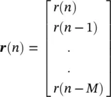

where M represents the finite impulse response (FIR) filter order. Conversely:

(4.112)

which can be simplified using the matrix inversion lemma [42]:

(4.113)

and finally, the update equation can be written as:

(4.114)

where

(4.115)

and the error e ( n ) after each iteration is recalculated as:

(4.116)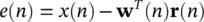

The second term in the right‐hand side of the above equation is . Presence of R −1( n ) in Eq. (4.115)is the major difference between RLS and LMS, but the RLS approach increases computation complexity by an order of magnitude.

All suboptimal transforms such as the DFT and DCT decompose the signals into a set of coefficients, which do not necessarily represent the constituent components of the signals. Moreover, the transform kernel is independent of the data hence they are not efficient in terms of both decorrelation of the samples and energy compaction. Therefore, separation of the signal and noise components is generally not achievable using these suboptimal transforms.

Expansion of the data into a set of orthogonal components certainly achieves maximum decorrelation of the signals. This enables separation of the data into the signal and noise subspaces.

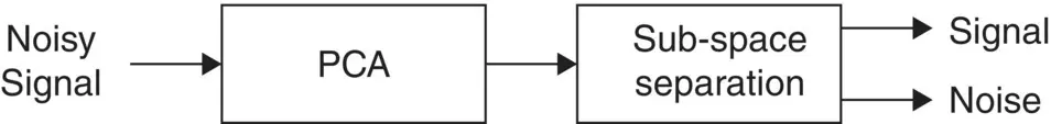
Figure 4.12 The general application of PCA.

For a single‐channel EEG the Karhunen–Loéve transform is used to decompose the i th channel signal into a set of weighted orthogonal basis functions:

(4.117)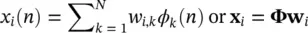

where Φ= { ϕ k} is the set of orthogonal basis functions. The weights w i, kare then calculated as:

(4.118)

Often noise is added to the signal, i.e. x i( n ) = s i( n ) + v i( n ), where v i( n ) is additive noise. This degrades the decorrelation process. The weights are then estimated in order to minimize a function of the error between the signal and its expansion by the orthogonal basis, i.e. e i= x i− Φw i. Minimization of the error in this case is generally carried out by solving the least‐squares problem. In a typical application of PCA as depicted in Figure 4.12, the signal and noise subspaces are separated by means of some classification procedure.

Singular value decomposition (SVD) is often used for solving the least‐squares (LS) problem. This is performed by decomposition of the M × M square autocorrelation matrix Rinto its eigenvalue matrix Λ= diag (λ 1, λ 2, … λ M) and an M × M orthogonal matrix of eigenvectors V, i.e. R = VΛV H, where (.) Hdenotes Hermitian (conjugate transpose) operation. Moreover, if Ais an M × M data matrix such that R= A H Athen there exist an M × M orthogonal matrix U, an M × M orthogonal matrix V, and an M × M diagonal matrix ∑with diagonal elements equal to , such that:

(4.119)

Hence ∑ 2= Λ.The columns of Uare called left singular vectors and the rows of V Hare called right singular vectors. If Ais rectangular N × M matrix of rank k then Uwill be N × N and ∑will be:

(4.120)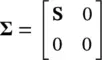

where S= diag (σ 1, σ 2, … σ k), where σ i= . For such a matrix the Moore–Penrose pseudo‐inverse is defined as an M × N matrix A †defined as:

(4.121)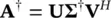

where ∑ †is an M × N matrix defined as:

(4.122)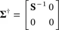

A †has a major role in the solutions of least‐squares problems, and S −1is a k × k diagonal matrix with elements equal to the reciprocals of the singular values of A, i.e.