Iain Pardoe - Applied Regression Modeling

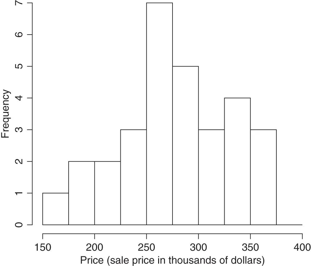
Figure 1.1Histogram for home prices example.

Histograms can convey very different impressions depending on the bin width, start point, and so on. Ideally, we want a large enough bin size to avoid excessive sampling “noise” (a histogram with many bins that looks very wiggly), but not so large that it is hard to see the underlying distribution (a histogram with few bins that looks too blocky). A reasonable pragmatic approach is to use the default settings in whichever software package we are using, and then perhaps to create a few more histograms with different settings to check that we are not missing anything. There are more sophisticated methods, but for the purposes of the methods in this book, this should suffice.

In addition to graphical summaries such as the stem‐and‐leaf plot and histogram, sample statistics can summarize data numerically. For example:

The sample mean, , is a measure of the “central tendency” of the data ‐values.

The sample standard deviation, , is a measure of the spread or variation in the data ‐values.

We will not bother here with the formulas for these sample statistics. Since almost all of the calculations necessary for learning the material covered by this book will be performed by statistical software, the book only contains formulas when they are helpful in understanding a particular concept or provide additional insight to interested readers.

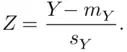
We can calculate sample standardized ‐values from the data ‐values:

Sometimes, it is useful to work with sample standardized ‐values rather than the original data ‐values since sample standardized ‐values have a sample mean of 0 and a sample standard deviation of 1. Try using statistical software to calculate sample standardized ‐values for the home prices data, and then check that the mean and standard deviation of the ‐values are 0 and 1, respectively.

Statistical software can also calculate additional sample statistics, such as:

the median (another measure of central tendency, but which is less sensitive than the sample mean to very small or very large values in the data)—half the dataset values are smaller than this quantity and half are larger;

the minimum and maximum;

percentiles or quantiles such as the 25th percentile—this is the smallest value that is larger than 25% of the values in the dataset (i.e., 25% of the dataset values are smaller than the 25th percentile, while 75% of the dataset values are larger).

Here are the values obtained by statistical software for the home prices example (see computer help #10):

Sample size,	Valid	30
	missing	0
Mean		278.6033
Median		278.9500
Standard deviation		53.8656
Minimum		155.5000
Maximum		359.9000
Percentiles	25	241.3750
	50	278.9500
	75	325.8750

There are many other methods—numerical and graphical—for summarizing data. For example, another popular graph besides the histogram is the boxplot ; see Chapter 6 ( www.wiley.com/go/pardoe/AppliedRegressionModeling3e) for some examples of boxplots used in case studies.

While the methods of the preceding section are useful for describing and displaying sample data, the real power of statistics is revealed when we use samples to give us information about populations . In this context, a population is the entire collection of objects of interest, for example, the sale prices for all single‐family homes in the housing market represented by our dataset. We would like to know more about this population to help us make a decision about which home to buy, but the only data we have is a random sample of 30 sale prices.

Nevertheless, we can employ “statistical thinking” to draw inferences about the population of interest by analyzing the sample data. In particular, we use the notion of a model —a mathematical abstraction of the real world—which we fit to the sample data. If this model provides a reasonable fit to the data, that is, if it can approximate the manner in which the data vary, then we assume it can also approximate the behavior of the population. The model then provides the basis for making decisions about the population, by, for example, identifying patterns, explaining variation, and predicting future values. Of course, this process can work only if the sample data can be considered representative of the population. One way to address this is to randomly select the sample from the population. There are other more complex sampling methods that are used to select representative samples, and there are also ways to make adjustments to models to account for known nonrandom sampling. However, we do not consider these here—any good sampling textbook should cover these issues.

Sometimes, even when we know that a sample has not been selected randomly, we can still model it. Then, we may not be able to formally infer about a population from the sample, but we can still model the underlying structure of the sample. One example would be a convenience sample —a sample selected more for reasons of convenience than for its statistical properties. When modeling such samples, any results should be reported with a caution about restricting any conclusions to objects similar to those in the sample. Another kind of example is when the sample comprises the whole population. For example, we could model data for all 50 states of the United States of America to better understand any patterns or systematic associations among the states.

Since the real world can be extremely complicated (in the way that data values vary or interact together), models are useful because they simplify problems so that we can better understand them (and then make more effective decisions). On the one hand, we therefore need models to be simple enough that we can easily use them to make decisions, but on the other hand, we need models that are flexible enough to provide good approximations to complex situations. Fortunately, many statistical models have been developed over the years that provide an effective balance between these two criteria. One such model, which provides a good starting point for the more complicated models we consider later, is the normal distribution .