Urban Remote Sensing

The resulting dDHM (see ahead to Figures 2.6and 2.7for examples) rapidly visualizes the extreme changes within the urban environment, namely newly constructed or demolished buildings. The differences identified are then summarized a number of different ways (e.g. amount of built‐up volume increase between t 1 and t 2, net increase/decrease of built‐up volume). Other approaches attach height and/or volumes attributes to multi‐temporal building footprints for a discrete vector analysis of change. Types of changes (e.g. from vegetation to building, building to demolished building) are characterized using criteria such as roof pitches/slopes, volumetric change metrics, and other parameters (Teo and Shih 2013; Dong et al. 2018). Multi‐temporal lidar analyses though, like any change detection work within remote sensing, are not without challenges and limitations. Specifically, comparison of multiple datasets is difficult when different data acquisition parameters (e.g. point densities, number of returns, time of year), data are pre‐processed and only provided in raster format (i.e. line‐up issues between datasets that must be resolved), lack of available ancillary datasets, and more.

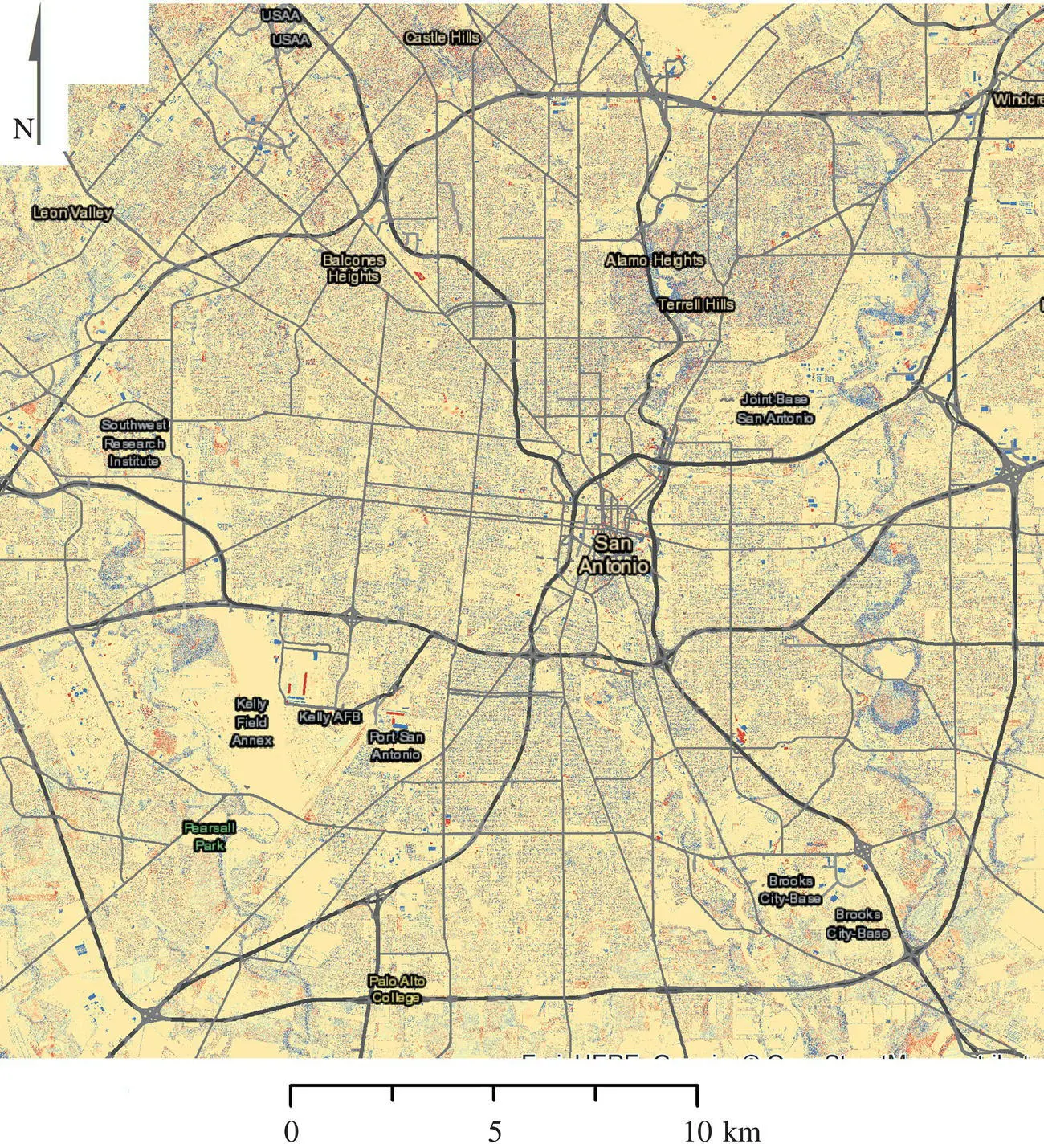
FIGURE 2.7 Citywide built‐up change (shown with dDHM) in San Antonio, Texas, 2003–2013 shown with blue indicating increased height values (i.e. new build‐up) and red decreased height values (i.e. demolished buildings). Vegetation is included in this example.

Texas cities have undergone tremendous growth over the past several decades. Unlike other US cities that have witnessed population stagnation or decline (e.g. Detroit, Buffalo), cities such as San Antonio have undergone a 34% increase in population in less than two decades; from 1.1 million residents in 2000 to 1.5 million by 2018 (US Census 2019). Subsequently, such changes are reflected on the urban landscape through residential development (e.g. housing, apartment building) and growth of retail/commercial spaces. Multi‐temporal lidar data provide an ideal geospatial dataset with which to identify such changes in 3D space; in this brief case study, we use lidar‐derived 1 m spatial resolution raster data provided by the Army Geospatial Center collected during the summer months (leaf‐on conditions) in 2003 and 2012.

As an example of 3D change in an urban area, Figure 2.6shows change in a commercial/retail space in southeast San Antonio between 2003 and 2012. When visually compared, the 2003 and 2012 DHMs (a and b respectively) indicate the removal of a large commercial building at the center and new build‐up in a portion of the space. When differenced via a dDHM, a single dataset can display the change including the type of change. For instance, Figure 2.6c shows the large building from 2003 in red that was demolished by 2012 where new build‐up is shown with blue. Interestingly, the dDHM reveals built‐up “ghosts” (red) that formerly dominated the urban landscape.

At the city‐scale ( Figure 2.7), the dDHM highlights extreme (large area) changes well. In this case, many large buildings removed between 2003 and 2012 (red) are visible west/southwest of downtown and along the interstate southeast of downtown. New build‐up (blue) is especially prevalent along the highways in the east/northeast and north parts of the city. At this scale though, much of the change, which covers small areas, is indistinguishable. During this period, much of the northern area shown in Figure 2.7was developed for residential land use, which can only partially be seen at this scale. In total, the dDHM‐based summation of volumetric change resulted in a net increase of around 27 Mm 3over this nine‐year period. Vegetation is included in this example and becomes apparent along the eastern extent of the analysis area stretching from north‐to‐south where tree canopy increased in size (some of this is a data artifact due to the 2012 data containing more vegetation points). In this way, dDHM calculation will reveal the changes in the urban environment but often not without also unveiling underlying data issues. In this example, because we did not have access to the raw lidar data, line‐up issues identified false changes on the landscape (e.g. building edges). Preprocessing can attempt to remove this noise but is sometimes unable to fully alleviate the problem.

With the capability to make Earth observations regardless of cloud cover and solar lighting conditions, radars have been successfully applied to Earth science studies and practical applications. Fundamentally, radar backscatter signatures are contributed by surface scattering such as from bare soil and bare ice, by a combination of surface and volume scattering such as from land surface with sparse and low vegetation cover, and by volume scattering such as from dense tropical forests (Ulaby et al. 1986; Tsang et al. 1985, and references therein). Specific to urban remote sensing, satellite radar data have been used to detect and observe urban characteristics in several cities (Henderson and Xia 1998; Dell'Acqua and Gamba 2006; Esch et al. 2009, 2017). Moreover, radars can delineate not only urban lateral extent in 2D but also building volume density in 3D (Nghiem et al. 2009; Mathews et al. 2019). The following subsections review the radar methodology applied to urban science research and applications.

The SeaWinds scatterometer aboard the QuikSCAT satellite (JPL 2006) was launched in June 1999 from the Space Launch Complex 4 (SLC‐4) at the Vandenberg Airforce Base in California, the United States. By definition, a scatterometer is a stable and accurate radar that can measure radar backscatter representing the ratio of the radar signal returned from a target on the Earth over the transmitted signal, expressed in decibels (dB). The QuikSCAT SeaWinds scatterometer had a swath width of 1400 km for the horizontal polarization and 1800 km for the vertical polarization with a nearly daily global coverage of the Earth. Radar backscatter data at each polarization were acquired in antenna conical scans in the full 360° azimuth with a constant incidence angle. QuikSCAT collected data at a Ku‐Band frequency of 13.4 GHz over both land and ocean for more than a decade from 1999 to 2009. With frequent temporal observations, QuikSCAT has a low spatial resolution due to the antenna large footprint in an “egg” shape of 25 km in azimuth and 37 km in range, which is too large for urban remote sensing. Thus, a method was developed to use multiple data collections over a longer period to obtain radar observations at a 1 km grid that is applicable to urban scales. This approach, the Dense Sampling Method (DSM), is summarized in the next subsection to explain how the temporal resolution is traded off for urban monitoring throughout the decade of the 2000s.

We provide a summary of the DSM but direct readers to the published literature for more mathematical and algorithmic details (Nghiem et al. 2009). First, QuikSCAT egg data are processed by a fast Fourier transform accounting for the Doppler compensation to generate a sub‐footprint thin “slice” data with a resolution of 6 km in range and 25 km in azimuth. For a given location on Earth, QuikSCAT slice data are densely collected annually and posted at 1/120° (~1 km at the equator) in the latitude‐longitude geographic projection. Then, a mathematical transformation, the Rosette Transform, is applied to calculate an ensemble average of slice backscatter values, denoted as and expressed by