Urban Remote Sensing
Здесь есть возможность читать онлайн «Urban Remote Sensing» — ознакомительный отрывок электронной книги совершенно бесплатно, а после прочтения отрывка купить полную версию. В некоторых случаях можно слушать аудио, скачать через торрент в формате fb2 и присутствует краткое содержание. Жанр: unrecognised, на английском языке. Описание произведения, (предисловие) а так же отзывы посетителей доступны на портале библиотеки ЛибКат.
- Название:Urban Remote Sensing
- Автор:
- Жанр:
- Год:неизвестен
- ISBN:нет данных
- Рейтинг книги:4 / 5. Голосов: 1
-
Избранное:Добавить в избранное
- Отзывы:
-
Ваша оценка:
Urban Remote Sensing: краткое содержание, описание и аннотация
Предлагаем к чтению аннотацию, описание, краткое содержание или предисловие (зависит от того, что написал сам автор книги «Urban Remote Sensing»). Если вы не нашли необходимую информацию о книге — напишите в комментариях, мы постараемся отыскать её.
is a state-of-the-art review of the latest progress in the subject. The text examines how evolving innovations in remote sensing allow to deliver the critical information on cities in a timely and cost-effective way to support various urban management activities and the scientific research on urban morphology, socio-environmental dynamics, and sustainability.
Chapters are written by leading scholars from a variety of disciplines including remote sensing, GIS, geography, urban planning, environmental science, and sustainability science, with case studies predominately drawn from North America and Europe.
A review of the essential and emerging research areas in urban remote sensing including sensors, techniques, and applications, especially some critical issues that are shifting the directions in urban remote sensing research. Illustrated in full color throughout, including numerous relevant case studies and extensive discussions of important concepts and cutting-edge technologies to enable clearer understanding for non-technical audiences.
will be of particular interest to upper-division undergraduate and graduate students, researchers and professionals working in the fields of remote sensing, geospatial information, and urban & environmental planning.
Urban Remote Sensing — читать онлайн ознакомительный отрывок
Ниже представлен текст книги, разбитый по страницам. Система сохранения места последней прочитанной страницы, позволяет с удобством читать онлайн бесплатно книгу «Urban Remote Sensing», без необходимости каждый раз заново искать на чём Вы остановились. Поставьте закладку, и сможете в любой момент перейти на страницу, на которой закончили чтение.
Интервал:
Закладка:
(2.3) 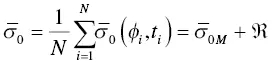
where N is the total number of slice data centered at the given location, and  is the backscatter value measured at time t iand azimuth direction φ iof each slice. In (2.1),
  is the mean part obtained by the Rosette Transform, and ℜ is the residual from the zero‐mean fluctuating part of the radar backscatter. In an urban area with stationary buildings and structures that have strong radar return,
  has a large and stable value ℜ while becoming small with a sufficiently large number of samples collected over a year (Nghiem et al. 2009). DSM backscatter provides a method to observe urban spatial pattern and temporal change based on physical structure in 3D, such as houses, factories, industrial plants, commercial centers, freeways, bridges, etc. As such, it is a crucial input to physical‐based climate‐urban nested modeling to assess impacts of urbanization (Jacobson et al. 2015, 2019), in contrast to urban extent arbitrarily demarcated based on administrative, legislative, and/or political arrangements (Taubenböck et al. 2019).
Notably, recent works have validated the capability of QuikSCAT data processed using the DSM for built‐up volume estimation in urban areas (Nghiem et al. 2017; Mathews et al. 2019). As an example, high DSM backscatter values for the Los Angeles area (see Figure 2.8a) exhibit a similar spatial pattern with high amounts of urban built‐up volume ( Figure 2.8b shown with individual building extents – i.e. clipped by building footprints). Similarly, the building volume and DSM patterns across large areas such as Austin, Texas ( Figure 2.9) are nearly indistinguishable, demonstrating the capability of DSM to capture 3D building volume structures in the city (Nghiem et al. 2017).
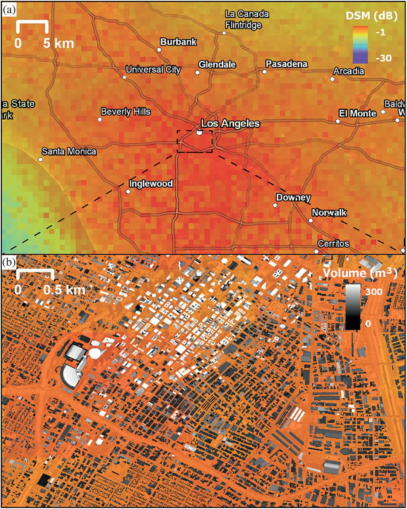
FIGURE 2.8 Pattern of DSM backscatter for greater Los Angeles, California (a) with stronger backscatter response in areas with higher amounts of urban built‐up volume (red; see downtown) and a transition to orange/yellow for suburban and rural area. In the downtown area (b), greater building footprint volumes (white) are spatially collocated with higher backscatter values (dark orange, red).
To quantitatively evaluate the degree to which DSM data can account for urban built‐up volume, we compared DSM backscatter to lidar‐derived building volumes aggregated to the same scale (1 km grid). Specifically, QuikSCAT data were processed using the DSM to match the geographic extent of airborne lidar data for nine cities in the United States (see Table 2.1for extents): Atlanta, Austin, Buffalo, Detroit, Los Angeles, New Orleans, San Antonio, Tulsa, and Washington, DC. The DSM data collapsed one year's worth of observations into a single dataset gridded in a pixel size of ~1 km. The year of data matched the year of lidar data collection ( Table 2.1); the lidar data were captured on differing dates but all during leaf‐on conditions during the summer months.
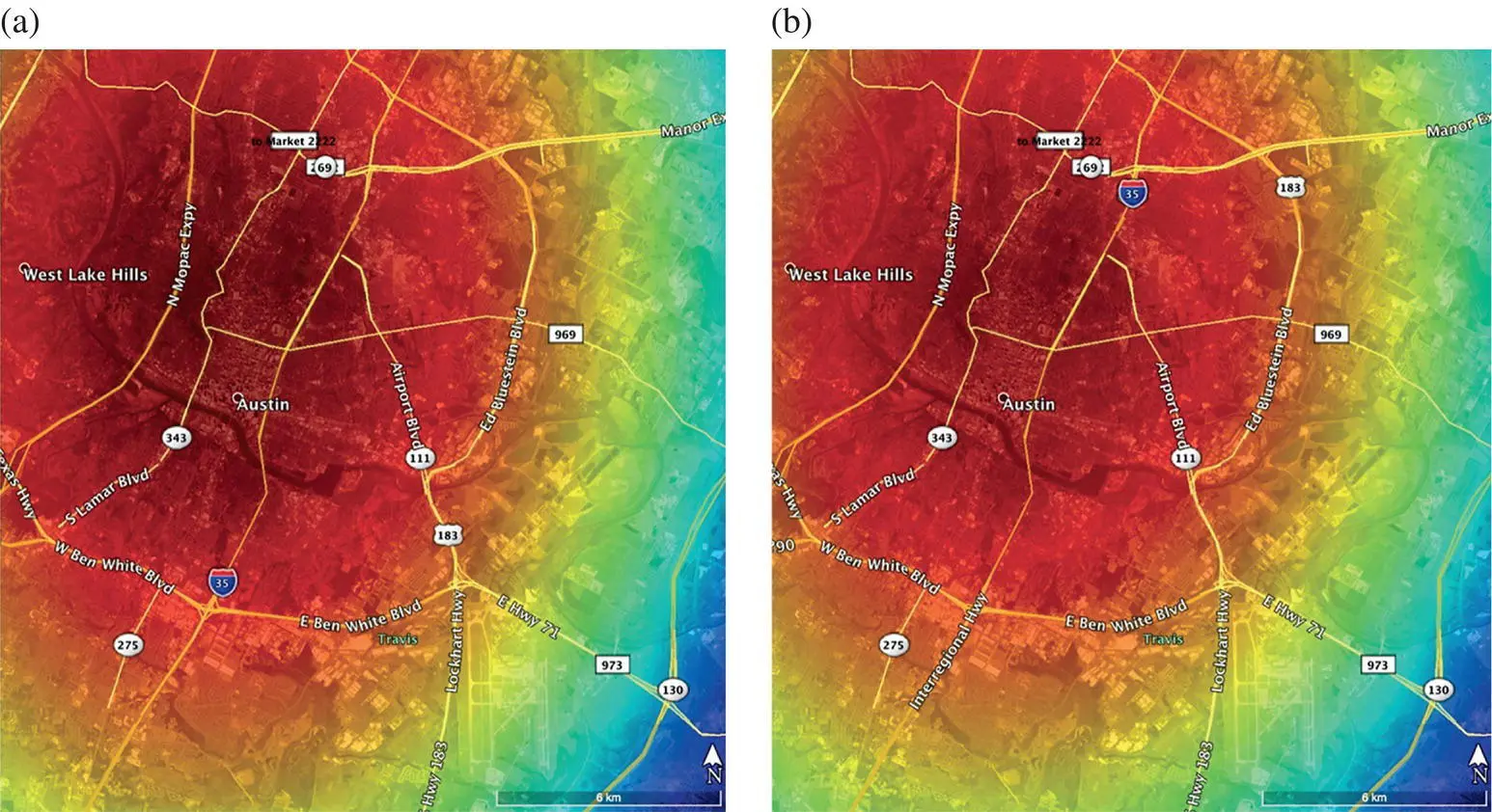
FIGURE 2.9 Spatial trend patterns for Austin, Texas in 2006 overlaid on Google Earth basemap. (a) The pattern of lidar‐derived building volume with the rainbow color scale from 0 to 9 Mm 3, and (b) the pattern of DSM radar backscatter with the rainbow color scale from −12 to −3 dB. The building volume and DSM patterns are nearly indistinguishable, demonstrating the capability of DSM to capture 3D building volume structures in the city (Nghiem et al. 2017).
Source : Nghiem et al. (2017).
Table 2.1 Coefficients of determination between DSM and lidar for nine US cities.
Source : Mathews et al. (2019)/Elsevier.
| City | Analysis year | Analysis extent (km 2) | DSM vs. lidar ( r 2) | DSM vs. lidar trend ( r 2) | DSM trend vs. lidar trend ( r 2) |
|---|---|---|---|---|---|
| Atlanta, GA | 2003 | 79 | 0.13 | 0.33 | 0.77 |
| Austin, TX | 2006 | 390 | 0.21 | 0.72 | 0.98 |
| Buffalo, NY | 2004 | 342 | 0.14 | 0.38 | 0.69 |
| Detroit, MI | 2004 | 347 | 0.10 | 0.52 | 0.81 |
| Los Angeles, CA a | 2007 | 64 | 0.04* | 0.26 | 0.64 |
| New Orleans, LA | 2008 | 346 | 0.04 | 0.21 | 0.33 |
| San Antonio, TX | 2003 | 640 | 0.20 | 0.75 | 0.97 |
| Tulsa, OK | 2008 | 1329 | 0.26 | 0.63 | 0.84 |
| Washington, DC | 2008 | 8297 | 0.32 | 0.66 | 0.98 |
Notes : r 2is coefficient of determination in linear model. All correlations significant with p ‐values < 0.01 unless otherwise noted (<0.05*).
aInsufficient data sample due to limited extent of lidar data.
The 1 m spatial resolution lidar‐derived raster data were provided by the Army Geospatial Center. Datasets included a DTM and two DSMs (first‐return and last‐return versions) for all cities that were used to generate a last‐return DHM (calculated as DTM minus the lastreturn DSM) with relative heights from the ground surface. The last‐return dataset was selected to avoid noise introduced by vegetation in areas with lower building heights (e.g. suburban areas where trees overhang buildings). Data fusion incorporating building footprints to clip out building‐only areas (i.e. remove noise) within cities ensured volume values are representative of only built‐up volume. The building footprint approach though does not include infrastructure such as highway overpasses and similar large nonbuilding features. Further, building footprint data are not always readily available (i.e. from local government), and take significant time to generate from scratch by way of GIS hand digitizing or OBIA. All nonbuilding pixels were reassigned values of zero. Per‐pixel volume (m 3) was then aggregated, summed, to match the 1 km spatial grid of the DSM data. The DSM and building volume values were then spatially coincident and prepared for statistical evaluation for measures of association, reported quantitatively as coefficients of determination or r 2. In addition, for comparison purposes, a spatial trend (see Şen 2017) of the data values for both the DSM and lidar was applied using the Trend tool in the ArcGIS Suite (e.g. DSM trend surface, lidar trend surface).
Results indicate a great deal of similarity between the DSM and lidar datasets. Figures 2.10and 2.11display two of the study cities, Tulsa and San Antonio, respectively, including all of the input datasets. The 1 km datasets illustrate the differences between the input data where the DSM ( Figures 2.10and 2.11c) is a smooth surface and the lidar version ( Figures 2.10and 2.11d) is much more discrete due to the extreme volume values representing the tallest buildings in the city's respective downtown and other highly built‐up areas. These differences provide visual confirmation of the differences between the two datasets and support the need for the spatial trend analysis. The spatial trend surfaces exhibit the same spatial patterns in terms of geographic extent and directionality of urban built‐up volume. The spatial trend concept is crucial as a quantitative representation of rural–urban transition that is a spatial change as a function of distance from the urban core (i.e. a spatial derivative). The spatial trend approach (Şen 2017) is mathematically robust, which circumvents the issue of taking spatial derivative of noisy discrete data of building structures, especially problematic and mathematically ill‐posed in very high‐resolution and thus very noisy data considering that buildings are typically vertical (e.g. 90° vertical walls) for which the derivative becomes infinitive or blows up. While many studies phrase the notion of rural–urban transition without a clear quantitative framework in a mathematically robust formulation, the DSM together with the spatial trend offers an elegant way to define and characterize rural–urban transition.
Читать дальшеИнтервал:
Закладка:
Похожие книги на «Urban Remote Sensing»
Представляем Вашему вниманию похожие книги на «Urban Remote Sensing» списком для выбора. Мы отобрали схожую по названию и смыслу литературу в надежде предоставить читателям больше вариантов отыскать новые, интересные, ещё непрочитанные произведения.


Обсуждение, отзывы о книге «Urban Remote Sensing» и просто собственные мнения читателей. Оставьте ваши комментарии, напишите, что Вы думаете о произведении, его смысле или главных героях. Укажите что конкретно понравилось, а что нет, и почему Вы так считаете.