Reservoir Characterization

It should be noted that the injected fluid in this experiment is CO 2supercritical, which has been injected under 1300 psi pressure and a temperature of 46 °C at a rate of 1 (ml/min) into the sample saturated with distilled water.

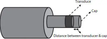
Figure 2.3 Schematic, placement of sample with transducer and the top cap.

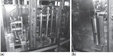
Figure 2.4 (a) The core flooding system, (b) Image of the holder connected to the core and transducers.

Travel times of compressional and shear waves through the super critically CO 2saturated core sample were measured at six different effective pressures (within the reservoir pressure range). Later on, corresponding compressional and shear wave velocities were calculated ( Figure 2.5).

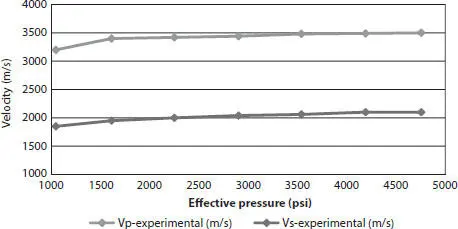
Figure 2.5 Compressional and shear wave velocity vs different effective pressure for super critically saturated core sample.

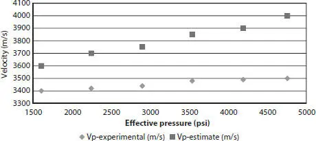
Figure 2.6 P-wave velocity (experimental and estimated) at different effective pressures.

To see how closely estimated wave velocity correlates with the experimental velocity values; we replaced the primary CO 2saturated water with brine (using apparent module of 2.25) using Gassmann equation. Then using the Greenberg-Castagna formula we estimated the compressional wave velocity ( Figure 2.6).

In Figure 2.6, the compressional wave velocity obtained from the laboratory experiment and the Gassmann equation is depicted versus effective pressure. It can be noticed that at all effective pressures the estimated velocities have higher values than experimental ones. The difference gradually enlarges as the effective pressure is increased. The rate of velocity increment is faster for estimated velocity than the experimental counterpart. This is because in Gassmann theory environment (the core) is considered a homogeneous and isotropic elastic environment. This theory is often true for Monomineralic rocks such as pure quartz sandstone or clean limestone. But since the sample used in this study developed naturally, possible impurities exist such as clay or fine cracks; so wave scattering is not considered in the Gassmann equations. It is also effective on bulk modulus and often in this hypothesis, it is assumed to be average. Another issue to the assumptions of this model is the fluid replacement instead of several fluids, regardless of their distribution in the environment and is often considered to be the average of the density of the fluids. This is effective on the accuracy of the model especially while the saturation is not uniform (Patchy saturation). Also with the pressure increasing, joints and cracks closed more and reduced permeability. Therefore, fluid flow and the opportunity to achieve balance are much reduced and the operating result is that Gassmann theory pushes farther than expected.

Shear wave velocity of the rock sample was determined at the different pressure from the estimated compressional wave velocity, using Greenberg-Castagna formulas.

Figure 2.7shows the experimental and estimated shear wave velocity values at different effective pressures. As it can be seen in contrary to the compressional wave, the estimated shear wave velocity is very much in accordance with the corresponding experimental values. Particularly this compatibility is more obvious at low effective pressures. The difference between experimental and estimated velocities and the rate of changes increase as the applied pressure increases. This is because the shear waves are only sensitive to changes solid in the environment. With the increase in effective pressure and reduced porosity and micro cracks, stone resistance increases against deformation (while volume or angle); as a result, it will face increasing shear wave velocity. Since in Greenberg-Castagna equation compressional and shear wave communication waves can be described with porosity and modules, effective stress plays an important role in the trend of estimation. But because of unconsidered pore shape, form, size, and density of fractures, anisotropy, texture and especially effective pressure on the environment in this relationship, differences although small can be seen in the results.

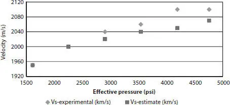
Figure 2.7 S-wave velocity (experimental and estimated) at different effective pressures.

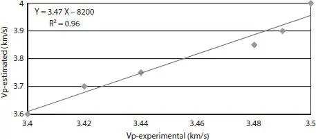
Figure 2.8 Cross plot of estimated P-wave velocities vs. laboratory measurements.

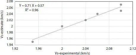
Figure 2.9 Cross plot of the estimated S-wave velocities vs. laboratory measurements.

Figure 2.8shows cross plot of the compressional wave velocity measured in the laboratory condition vs. the estimated values along with a best-fitted line. The correlation of the values is 0.95. Figure 2.9also shows the cross plot of the experimental and estimated shear wave velocities along with a best fitted line. The correlation of the values is 0.96.

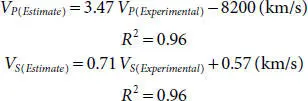
Figures 2.10and 2.11show the cross plots of the experimental and estimated compressional and shear wave velocities. Mathematical relationship between two sets of wave velocities were obtained. As it shows 90% correlation observed in both modes between compressional and shear wave velocity. The important note is that the slope of the curve is approximately 5 times in the experimental measurements more than the estimated measurement and this is due to larger estimated compressional wave velocity.

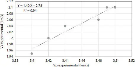
Figure 2.10 Plot of experimental shear wave velocity against compressional wave velocity.

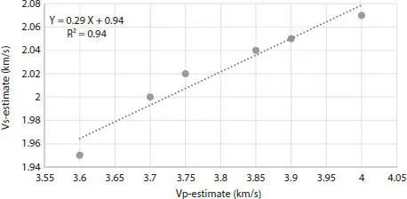
Figure 2.11 Plot of estimated shear wave velocity against compressional wave velocity.

Since Greenberg-Castagna model assumptions is ideal for a specially designed environment, there is no great match between this model and laboratory values. But as was mentioned earlier, correspondence between the velocity, the pressure and shear are very close together. It seems environment effective pressure is the essential factor that change is not considered in the model. This effect is highlighted on shear wave velocity and shear wave module.