Stephen Winters-Hilt - Informatics and Machine Learning

For prokaryotic gene prediction much of the problem with obtaining high‐confidence training data can be circumvented by using a bootstrap gene‐prediction approach. This is possible in prokaryotes because of their simpler and more compact genomic structure: simpler in that long ORFs are usually long genes, and compact in that motif searches upstream usually range over hundreds of bases rather than thousands (as in human).

Interpolated Markov Model (IMM) : the order of the MM can be interpolated according to a globally imposed cutoff criterion (see Figure 3.5), such as a minimum sub‐sequence count: fourth‐order passes if Counts ( x 0; x −1; x −2; x −3; x −4)>cutoff for all x −4… x 0sub‐sequences (100, for example), the utility of this becomes apparent with the following reexpression:

TotalCounts(length5)/TotalCounts(length4)

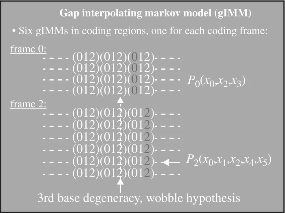
Figure 3.5 Hash interpolated Markov model (hIMM) and gap/hash interpolated Markov model (ghIMM): now no longer employ a global cutoff criterion – count cutoff criterion applied at the sub‐sequence level. Given the current state and the emitted sequence as x 1, …, x L; compute: P ( x L∣ x 1, …, x L − 1) ≈ Count( x 1, …, x L)/Count( x 1, …, x L − 1). If Count( x 1, …, x L − 1) ≥ 400 i.e. only if the parental sequence shows statistical significance (consider 400 = 4 × 100, or requiring >100 counts on observations assuming uniform distribution for count cutoff determination), store P ( x L∣ x 1, …, x L − 1) in the hash. (If gene finding, have at least five states, e.g. need to maintain a separate hash for each of the following states – Junk, Intron, and Exon0, 1, 2.)

Suppose Counts ( x 0; x −1; x −2; x −3; x −4; x −5) x −5… x 0sub‐sequence, then the interpolation would halt (globally), and the order of MM used would be fourth‐order.

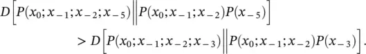
Gap Interpolated Markov Model (gIMM) : like IMM with its count cutoff, but when going to higher order in the interpolation there is no constraint to contiguous sequence elements – i.e. “gaps” are allowed. The resolution of what gap‐size to choose when going to the next higher order is resolved by evaluating the Mutual Information. i.e. when going to 3rd order in the Markov context, P ( x 0∣ x −5; x −2; x −1) is chosen over P ( x 0∣ x −3; x −2; x −1) if

Or, in terms of Kullback–Leibler divergences, if

1 3.1 In Section 3.1, the Maximum Entropy Principle is introduced. Using the Lagrangian formalism, find a solution that maximizes on Shannon entropy subject to the constraint of the “probabilities” sum to one.

2 3.2 Repeat the Lagrangian optimization of (Exercise 3.1) subject to the added constraint that there is a mean value, E(X) = μ.

3 3.3 Repeat the Lagrangian optimization of (Exercise 3.2) subject to the added constraint that there is a variance value, Var(X) = E(X2)(E(X))2 = σ2.

4 3.4 Using the two‐die roll probabilities from (Exercise 2.3) compute the mutual information between the two die using the relative entropy form of the definition. Compare to the pure Shannon definition: MI(X, Y) = H(X) + H(Y) – H(X, Y).

5 3.5 Go to genbank ( https://www.ncbi.nlm.nih.gov/genbank) and select the genomes of three medius‐sized bacteria (~1 Mb), where two bacteria are closely related. Using the Python code shown in Section 2.1, determine their hexamer frequencies (as in Exercise 2.5 with virus genomes). What is the Shannon entropy of the hexamer frequencies for each of the three bacterial genomes? Consider the following three ways to evaluate distances between the genome hexamer‐frequency profiles (denoted Freq(genome1), etc.), try each, and evaluate their performance at revealing the “known” (that two of the bacteria are closely related):distance = Shannon difference = | H(Freq(genome1))−H(Freq(genome2))|.distance = Euclidean distance = d(Freq(genome1),Freq(genome2)).distance = Symmetrized Relative Entropy= [D(Freq(genome1)||Freq(genome2))+D(Freq(genome2)||Freq(genome1))]/2Which distance measure provides the clearest identification of phylogenetic relationship? Typically it should be (iii).

6 3.6 Exercise 3.5, if done repeatedly, will eventually reveal that the best distance measure (between distributions) is the symmetrized relative entropy (case (iii)). Notice that this means that when comparing two distributions we quantify their difference not by a difference on Shannon entropies, case (i). In other words, we choose:Difference(X, Y) = MI(X, Y) = H(X) + H(Y) – H(X, Y),Not Difference = ∣ H(X) – H(Y)∣.The latter case satisfies the metric properties, including triangle inequality, in order to be a “distance” measure, is this true for the mutual information difference as well?

7 3.7 Go to genbank ( https://www.ncbi.nlm.nih.gov/genbank) and select the genome of the K‐12 strain of E. coli. (The K‐12 strain was obtained from the stool sample of a diphtheria patient in Palo Alto, CA, in 1922, so that seems like a good one.) Reproduce the MI codon discovery described in Figure 3.1.

8 3.8 Using the E. coli genome (the one described above) and using the codon counter code, get the frequency of occurrence of the 64 different codons genome‐wide (without even restricting to coding regions or to a particular “framing,” these are still unknowns, initially, in an ab initio analysis). This should reveal oddly low counts for what will turn out to be the “stop” codons.

9 3.9 Using the code examples with stops used to mark boundaries, identify long ORF regions in the E. coli genome (the one described in (Exercise 3.7)). Produce an ORF length histogram like that shown in Figure 3.2.

10 3.10 Create an overlap‐encoding topology scoring method (like that described for Figure 3.3), and use it to obtain topology histograms like those shown in Figure 3.3a and Figure 3.4. Do this for the following genomes: E. coli (K‐12 strain); V. cholera; and Deinococcus Radiodurans.

11 3.11 In a highly trusted coding region, such as the top 10% of the longest ORFs in the E. coli genome analysis, perform a gap IMM analysis, which should approximately reproduce the result shown in Figure 3.5.

12 3.12 Prove that relative entropy is always positive.

Текст предоставлен ООО «ЛитРес».

Прочитайте эту книгу целиком, купив полную легальную версию на ЛитРес.