Stephen Winters-Hilt - Informatics and Machine Learning

Before moving on to more sophisticated gene structure identification ( Chapter 4), let us first consider the multi‐frame and two‐strand aspect of the genomic information and what this might mean for the “topology” or overlap placement of coding regions. To recap, smORF offers information about ORFs, and tallies information about other such codon void regions (an ORF is a void in three codons: TAA, TAG, TGA). This allows for a more informed selection process when sampling from a genome, such that non‐overlapping gene starts can be cleanly and unambiguously sampled. Furthermore, overlapping ORF coding regions can be identified and enumerated (see Figures 3.3and 3.4).

The goal with smORF was, initially, to identify key gene structures (e.g. stop codons, etc.) and use only the highest confidence examples to train profilers. Once this was done, Markov models (MMs) were (bootstrap) constructed on the suspected start/stop regions and coding/noncoding regions. The algorithm then iterated again, informed with the MM information, and partly relaxes the high fidelity sampling restrictions (essentially, the minimum allowed ORF length is made smaller). A crude gene‐finder was then constructed on the high fidelity ORFs by use of a very simple heuristic: scan from the start of an ORF and stop at the first in‐frame “atg” (to be implemented in Chapter 4). This analysis was applied to the Vibrio cholerae genome (Chr. I). 1253 high fidelity ORFs were identified out of 2775 known genes. This first‐“atg” heuristic provided a gene prediction accuracy of 1154/1253 (92.1% of predictions of gene regions were exactly correct). If small shifts are allowed in the predicted position of the start‐codon relative to the first‐“atg” (within 25 bases on either side), then prediction accuracy improves to 1250/1253 (99.8%). This actually elucidates a key piece of information needed to improve such a prokaryotic gene‐finder: information is needed to help identify the correct start codon in a 50‐base window from the first ATG. Such information exists in the form of DNA motifs corresponding to the binding footprint of regulatory biomolecules (that play a role in transcriptional or translational control). Further bootstrap refinements along these lines are done in Chapter 4to produce an ab initio prokaryotic gene finder with 99.9% or better accuracy.

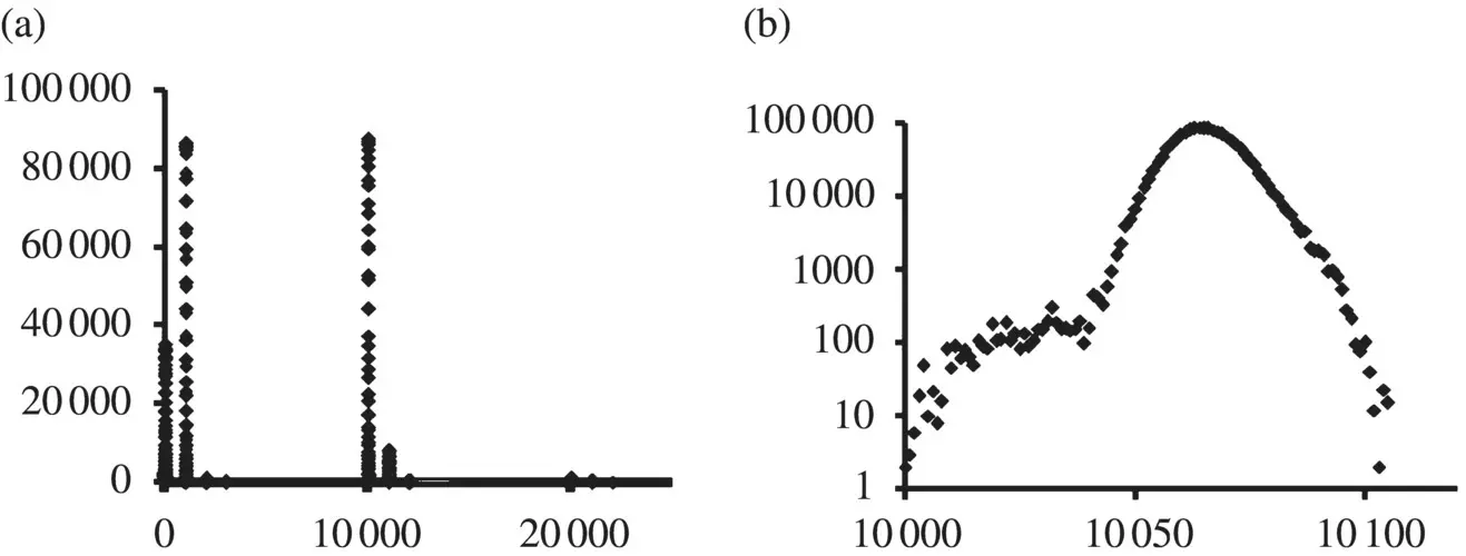
Figure 3.3 (a) Topology index histograms shown for the V. cholerae CHR. I genome, where the x ‐axis is the topology index, and the y ‐axis shows the event counts (i.e. occurrence of that particular topology index in the genome). The topology index is computed by the following scheme: (i) initialize index for all bases in sequence to zero. (ii) Each base in a forward sense ORF, with length greater than a specified cutoff, is incremented by +10 000 for each such ORF overlap. Similarly, bases in reverse sense ORFs are incremented by +1000 for each such overlap. Voids larger than the cutoff length in the nonstandard smORFs each give rise to an increment of +1. The top panel above shows that V. cholerae only has a small portion of its genome involved in multiple gene encodings. The (b) panel shows a “blow‐up” of the 10 000 peak.

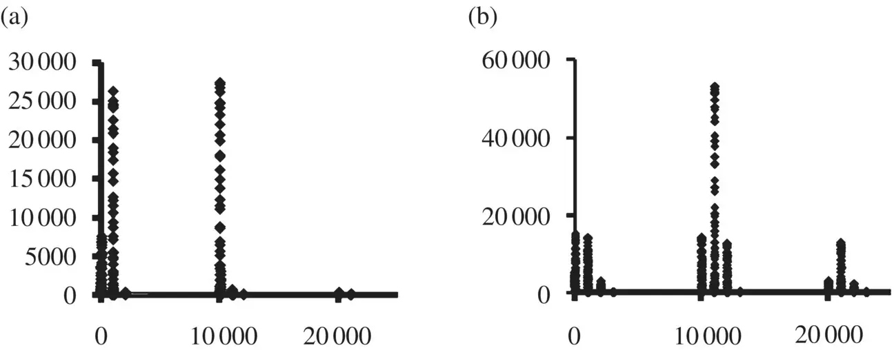
Figure 3.4 Topology‐index histograms are shown for the Chlamydia trachomatis genome,(a), and Deinococcus radiodurans genome, (b) C. trachomati s, like V. cholerae , shows very little overlapping gene structure. D. radiodurans , on the other hand, is dominated by genes that overlap other genes (note the strong 11 000 peak).

Ab initio gene‐finding can identify the stop codons and, thus, (standard) ORFs. A generalization to codon void regions, with all six frame passes, also leads to recognition of different, overlapping , potential gene regions (and then doubled given the two orientations). A genome‐topology scoring as shown in Figure 3.3can clearly show differences between bacteria ( Figure 3.4) – and is thus a possible “fingerprinting” tool.

The prokaryotic genome analysis is similar to both the prokaryotic and eukaryotic transciptome analysis (where eukaryotic transcriptome analysis is similar since the introns have been removed). The analysis tools for prokaryotic genomes, described thus far, are primarily what are needed for either prokaryotic or eukaryotic transcriptome analysis. Surprisingly, the same overlapping void topologies, with reverse overlap orientation (“duals”), are seen at transcriptome level in eukaryotes as in prokaryotes. For eukaryotic transcripts with overlaps that are “dual”, however, this has special significance. Recall that a transcript that encodes overlapping read direction “duality” (with regulatory regions intact and lengthy ORF size, so highly likely functional), is only from a single genome‐level pre‐messenger ribonucleic acid (mRNA) due to intron splicing in eukaryotes. This is a very odd arrangement (artifact) for eukaryotes unless they evolved from an ancient prokaryote as hypothesized in a number of theories where such an overlap topology would already be in place to “imprint thru.” The specific nature of this transcriptome artifact, however, is best explained via the viral eukaryogenesis hypothesis (see [1, 3]).

Just as Chapter 2finished with a Math review, we do the same again here in the context of sequential processes. The core mathematical tool for describing a sequential process (where limited memory suffices) is the Markov chain, so that will be defined first. In the context of genome analysis, however, the standard Markov chain based feature extraction is no longer optimal (especially given the nature of the computational resources). Thus, novel mathematical generalization of the Markov chain description, interpolated Markov models, will be given as well.The gap/hash interpolated Markov model, in particular, can be used to “vacuum‐up” all motif information in specified regions. This could be used and directly integrated into an HMM‐based gene finder ( Chapters 7and 8), or, alternatively, provide identification of a typical motif set for some circumstance (as will be done in Chapter 4).

A Markov chain is a sequence of random variables S 1; S 2; S 3; … with the Markov property of limited memory, where a first‐order Markov assumption on the probability for observing a sequence “ s 1 s 2 s 3 s 4… s n” is:

In the Markov chain model, the states are also the observables. For a HMM we generalize to where the states are no longer directly observable (but still first‐order Markov), and for each state, say S 1, we have a statistical linkage to a random variable, O 1, that has an observable base emission, with the standard (0th‐order) Markov assumption on prior emissions.

The key “short‐term memory” property of a Markov chain is: P ( x i∣ x i − 1, …, x 1) = P ( x i∣ x i − 1) = a i − 1, i, where a i − 1, iare sometimes referred to as “transition probabilities”, and we have: P ( x ) = P ( x L, x L − 1, …, x 1) = P ( x 1)∏ i = 2…L a i − 1, i. If we denote C yfor the count of events y , C xyfor the count of simultaneous events x and y , T yfor the count of strings of length one, and T xyfor the count of strings of length two: a i − 1, i= P ( x ∣ y ) = P ( x , y )/ P ( y ) = [ C xy/ T xy]/[ C y/ T y]. Note: since T xy+ 1 = T y→ T xy≅ T y(sequential data sample property if one long training block), a i − 1, i≅ C xy/ C y= C xy/∑ x C xy, so counts C xyis complete information for determining transition probabilities.