Benoîte de Saporta - Martingales and Financial Mathematics in Discrete Time

The σ -algebra generated by X represents all the events that can be observed by drawing X . It represents the information revealed by X .

DEFINITION 1.14.– Let (Ω, , ℙ) be a probability space .

– Let X and Y be two random variables on (Ω, , ℙ) taking values in (E1, ε1) and (E2, ε2). Then, X and Y are said to be independent if the σ-algebras σ(X) and σ(Y) are independent.

– Any family (Xi)i∈I of random variables is independent if the σ-algebras σ(Xi) are independent.

– Let be a sub-σ-algebra of , and let X be a random variable. Then, X is said to be independent of if σ(X) is independent of or, in other words, and are independent.

PROPOSITION 1.8.– If X and Y are two integrable and independent random variables, then their product XY is integrable and [ XY ] = [ X ] [ Y ].

We will now more closely study random variables taking values in ℝ d, with d ≥ 2. This concept has already been defined in Definition 1.9. We will now look at the relations between the random vector and its coordinates. When d = 2, we then speak of a random couple.

PROPOSITION 1.9.– Let X be a real random vector on the probability space (Ω, , ℙ), taking values in ℝ d . Then ,

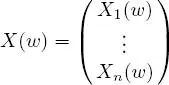
is such that for any i ∈ {1, ..., d }, X i is a real random variable .

DEFINITION 1.15.– A random vector is said to be discrete if each of its components, X i, is a discrete random variable .

DEFINITION 1.16.– Let be a discrete random couple such that

The conjoint distribution (or joint distribution or, simply, the distribution) of X is given by the family

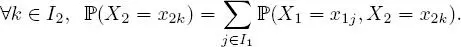
The marginal distributions of X are the distributions of X 1 and X 2 . These distributions may be derived from the conjoint distribution of X through:

and

The concept of joint distributions and marginal distributions can naturally be extended to vectors with dimension larger than 2.

EXAMPLE 1.21.– A coin is tossed 3 times, and the result is noted. The universe of possible outcomes is Ω = { T, H } 3 . Let X denote the total number of tails obtained and Y denote the number of tails obtained at the first toss. Then ,

The couple ( X, Y ) is, therefore, a random vector (referred to here as a “random couple”), with joint distribution defined by

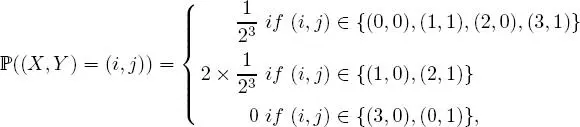
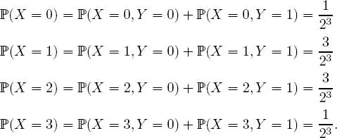
for any ( i, j ) X (Ω) × Y (Ω), which makes it possible to derive the distributions of X and Y (called the marginal distributions of the couple ( X, Y ) ):

Distribution of X:

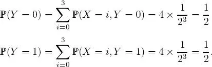
Distribution of Y :

To conclude this section on random variables, we will review some classic results of convergence for sequences of random variables. Throughout the rest of this book, the abbreviation r.v . signifies random variable .

DEFINITION 1.17.– Let ( X n) n≥1 and X be r.v.s defined on (Ω, , ℙ).

1 1) It is assumed that there exists p > 0 such that, for any n ≥ 0, [|Xn|p] < ∞, and [|X|p] < ∞. It is said that the sequence of random variables (Xn)n≥1 converges on the average of the order p or converges in Lp towards X, ifWe then write In the specific case where p = 2, we say there is a convergence in quadratic mean.

2 2) The sequence of r.v. (Xn)n≥1 is called almost surely (a.s.) convergent towards X, if

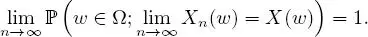
We then write

THEOREM 1.1 (Monotone convergence theorem).– Let ( X n) n≥1 be a sequence of positive and non-decreasing random variables and let X be an integrable random variable, all of these defined on the same probability space (Ω, P) . If ( X n) converges almost surely to X, then

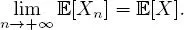
THEOREM 1.2 (Dominated convergence theorem).– Let ( X n) n≥1 be a sequence of random variables and let X be another random variable, all defined on the same probability space (Ω, , ℙ) . If the sequence ( X n) converges to X a.s., and for any n ≥ 1, | X n|≤ Z, where Z is an integrable random variable, then and, in particular ,