Benoîte de Saporta - Martingales and Financial Mathematics in Discrete Time

The following proposition establishes a link between the expectation of a discrete, random variable and measure theory.

PROPOSITION 1.3.– Let X be a discrete random variable such that X (Ω) = { x i, i ∈ I }, where I ⊂ ℕ . It is assumed that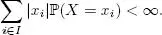

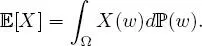
Then ,

The above proposition also justifies the concept of integrability introduced in Definition 1.12. Further, in this case (i.e. when X is integrable: 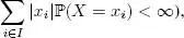we write X ∈ L 1(Ω, , ℙ).

When X pis integrable for a certain real number p ≥ 1 (i.e. when we write

Let us look at some of the properties of expectations.

PROPOSITION 1.4.– Let X and Y be two integrable, discrete random variables, a, b ∈ ℝ . Then ,

1 1) Linearity: [aX + bY ] = a[X]+ b[Y ].

2 2) Transfer theorem: if g is a measurable function such that g(X) is integrable, then

3 3) Monotonicity: if X ≤ Y almost surely (a.s.), then [X] ≤ [Y].

4 4) Cauchy–Schwartz inequality: If X2 and Y2 are integrable, then XY is integrable and

5 5) Jensen inequality: if g is a convex function such that g(X) is integrable, then,

DEFINITION 1.13.– Let X be a discrete random variable, such that X (Ω) = { x i, i ∈ I }, I ⊂ ℕ and X 2 is integrable. The variance of X is the real number:

Variance satisfies the following properties.

PROPOSITION 1.5.– If a discrete random variable X admits variance, then ,

1 1) (X) ≥ 0.

2 2) (X) = [X2] − ([X])2.

3 3) For any (a, b) ∈ ℝ2, (aX + b) = a2(X).

We now define the σ -algebra generated by a random variable. This concept is important for several reasons. For instance, it can make it possible to define the independence of random variables. It is also at the heart of the definition of conditional expectations; see Chapter 2.

PROPOSITION 1.6.– Let X be a real random variable, defined on (Ω, , ℙ) taking values in ( E , ε ) . Then , X= X −1( ε ) = { X −1( A ); A ∈ ε} is a sub-σ-algebra of on Ω . This is called the σ-algebra generated by the random variable X. It is written as σ ( X ) . It is the smallest σ-algebra on Ω that makes X measurable:

EXAMPLE 1.19.– Let 0= {∅, Ω} and X = c ∈ ℝ be a constant. Then, for any Borel set B in ℝ, ( X ∈ B ) has the value ∅ if c ∉ B and Ω if c ∈ B. Thus, the σ-algebra generated by X is 0 . Reciprocally, it can be demonstrated that the only 0 -measurable random variables are the constants. Indeed, let X be a 0 -measurable random variable. Assume that it takes at least two different values, x and y. It may be assumed that y ≥ x without loss of generality. Therefore , We have that ( X ∈ B ) is non-empty because x ∈ B but is not Ω since y ∉ B. Therefore, X is not 0 -measurable .

PROPOSITION 1.7.– Let X be a random variable on (Ω, , ℙ) taking values in ( E , ε ) and let σ ( X ) be the σ-algebra generated by X. Thus, a random variable Y is σ ( X ) -measurable if and only if there exists a measurable function f such that Y = f ( X ).

This technical result will be useful in certain demonstrations further on in the text. In general, if it is known that Y is σ ( X )-measurable, we cannot (and do not need to) make explicit the function f . Reciprocally, if Y can be written as a measurable function of X , it automatically follows that Y is σ ( X )-measurable.

EXAMPLE 1.20.– A die is rolled 2 times. This experiment is modeled by Ω = {1, 2, 3, 4, 5, 6} 2 endowed with the σ-algebra of its subsets and the uniform distribution. Consider the mappings X 1, X 2 and Y from Ω onto ℝ defined by

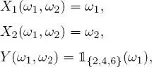
thus, X i is the result of the ith roll and Y is the parity indicator of the first roll. Therefore, thus, Y is σ ( X 1) -measurable. On the other hand, Y cannot be written as a function of X 2.