Benoîte de Saporta - Martingales and Financial Mathematics in Discrete Time

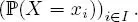
EXAMPLE 1.13.– Uniform distribution: Let and { x 1, ..., x N} ⊂ ℝ . Let X be a random variable on (Ω, , ℙ) such that X (Ω) = { x 1, ..., x N} and for any i ∈ {1, ..., N },

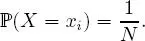
It is then said that X follows a uniform distribution on { x 1, ..., x N}.

EXAMPLE 1.14.– The Bernoulli distribution: Let p ∈ [0, 1] . Let X be a random variable on (Ω, , ℙ) such that X (Ω) = {0, 1} and

It is then said that X follows a Bernoulli distribution with parameter p, and we write X ∼ ( p ).

The Bernoulli distribution models random experiments with two possible outcomes: success, with probability p, and failure, with probability 1 – p. This is the case in the following game. A coin is tossed N times. This experiment is modeled by Ω = { T, H } N, endowed with the σ-algebra of its subsets and the uniform distribution. For 1 ≤ n ≤ N, the mappings X n from Ω onto ℝ are considered, defined by

the number of tails at the nth toss. Thus, X n, 1 ≤ n ≤ N, are random real variables in the Bernoulli distribution with parameter 1 / 2 if the coin is balanced .

EXAMPLE 1.15.– Binomial distribution: Let p ∈ [0, 1], and X be a random variable on (Ω, , ℙ) such that X (Ω) = {0, 1, ..., N } and for any k ∈ {0, 1, ..., N },

It is then said that X follows a binomial distribution with parameters N and p, and we write X ∼ ( N, p ).

If the Bernoulli experiment with probability of success p is repeated N times, independently, then the binomial distribution is the distribution of the random variable containing the number of successes at the end of the N repetitions of the experiment .

EXAMPLE 1.16.– Hypergeometric distribution: Let n and N be two integers such that n ≤ N, p ∈]0, 1[ such that pN ∈ ℕ, and let X be a random variable on (Ω, , ℙ) such that

and for any k ∈ X (Ω),

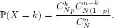
X is then said to follow a hypergeometric distribution with parameters N, n and p, and we write X ∼ ( N, n, p ).

If we consider an urn containing N indistinguishable balls, k red balls and N – k white balls, with k ∈ {1, ...N 1}, and if we simultaneously draw n balls, then the random variable X, equal to the number of red balls obtained, follows a hypergeometric distribution with parameters N, n and

EXAMPLE 1.17.– Poisson distribution: Let λ > 0 and X be a random variable on (Ω, , ℙ) such that

and for any k ∈ X (Ω),

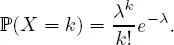
It is then said that X follows a Poisson distribution with parameter λ, and we write X ∼ ( λ ).

DEFINITION 1.12.– Let X be a discrete random variable such that X (Ω) = { x i, i ∈ I }, where I ⊂ ℕ.

– X or the distribution of X is said to be integrable (or summable) if

– If X is integrable, then the expectation of X is the real number defined by

EXAMPLE 1.18.– The random variable X defined in Example 1.12 admits an expectation equal to

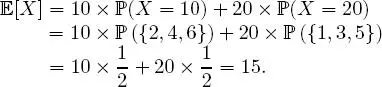
The average winnings in the die-rolling game is therefore equal to 15 .