Benoîte de Saporta - Martingales and Financial Mathematics in Discrete Time

– If (An)n∈ℕ is decreasing (for the inclusion), then,

We will now review the concept of independent events and σ -algebras.

DEFINITION 1.8.– Let (Ω, , ℙ) be a probability space .

– Two events, A and B, are independent if ℙ(A ∩ B) = ℙ(A) × ℙ(B).

– A family of events (Ai ∈ i, i ∈ I) is said to be mutually independent if for any finite family J ⊂ I, we have

– Two σ-algebras and are independent if for any A ∈ and B ∈ , A and B are independent.

– A family of sub-σ-algebra i ⊂ , i ∈ I is mutually independent if any family of events (Ai ∈ i, i ∈ I) is mutually independent.

EXAMPLE 1.10.– We roll a six-faced die and write

– A1 the event “the number obtained is even”; and

– A2 the event “the number obtained is a multiple of 3” .

The universe of possible outcomes is Ω = {1, 2, 3, 4, 5, 6} which has a finite number of elements and as all its elements have the same chance of occurring, we can endow it with the uniform probability . Since

we have

Therefore, A 1 and A 2 are two independent events .

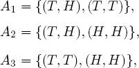
EXAMPLE 1.11.– A coin is tossed twice. The following events are considered:

– A1 “Obtaining tails (T) on the first toss”;

– A2 “Obtaining heads (H) on the second toss”; and

– A3 “Obtaining the same face on both tosses”.

The universe of possible outcomes is

which has four elements, and as all elements have the same chance of occurring, it can be endowed with uniform probability. Since

we have

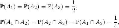
and Thus, the events A 1, A 2 and A 3 are pairwise independent, but are not mutually independent. Unless specified, the notion of independence by default always signifies mutual independence and not pairwise independence .

Let us now recall the definition of a generic random variable, and then the specific case of discrete random variables.

DEFINITION 1.9.– Let (Ω, , ℙ) be a probabilizable space and ( E , ε ) be a measurable space. A random variable on the probability space (Ω, , ℙ) taking values in the measurable space ( E , ε ), is any mapping X : Ω → E such that, for any B in ε, X −1( B ) ∈ ; in other words, X : Ω → E is a random variable if it is an ( , ε ) -measurable mapping. We then write the event “ X belongs to B ” by

In the specific case where E = ℝ and = ε = (ℝ), the mapping X is called a real random variable. If E = ℝ d with d ≥ 2, and ε = (ℝ d), the mapping X is said to be a real random vector .

EXAMPLE 1.12.– Let us return to the experiment where a six-sided die is rolled, where the set of possible outcomes is Ω = {1, 2, 3, 4, 5, 6}, which is endowed with the uniform probability. Consider the following game:

– if the result is even, you win 10 ;

– if the result is odd, you win 20 .

This game can be modeled using the random variable defined by:

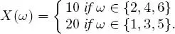
This mapping is a random variable, since for any B ∈ ({10, 20}), we have

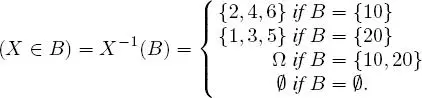
and all these events are in (Ω).

DEFINITION 1.10.– The distribution of a random variable X defined on (Ω, , ℙ) taking values in ( E , ε ) is the mapping ℙ X: ε → [0, 1] such that, for any B ∈ ε,

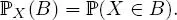
The distribution of X is a probability distribution on ( E , ε ) ; it is also called the image distribution of ℙ by X .

DEFINITION 1.11.– A random real variable is discrete if X (Ω) is at most countable. In other words, if X (Ω) = x i, i ∈ I , where I ⊂ ℕ . In this case, the probability distribution of X is characterized by the family