Geophysical Monitoring for Geologic Carbon Storage

We build a 1D velocity model for this site based on geological layers and previous seismic refraction survey in this area (Walter & Mooney, 1987; Birkholzer et al., 2011). Layers with thickness less than 200 m are merged with their neighboring layers to create a simple model. Figure 4.3shows the layered P‐wave velocity model. The S‐wave velocity model is similar to the P‐wave velocity model with a V P/ V S= 1.73.

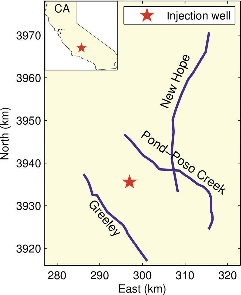
Figure 4.2 The location of the Kimberlina CCUS (carbon capture, utilization, and storage) pilot site. Major faults are shown as blue lines. The red star is the location of the injection well.

For a synthetic demonstration, we take a portion of the Pond‐Poso Creek Fault, and study the optimal design of surface seismic network for microseismic monitoring. The Pond‐Poso Creek Fault is a kilometer‐wide zone of northwesterly striking normal faults with large dip angles. For simplicity, we assume the fault is vertical. We create hundreds of microseismic events on the fault from depths between 1 km to 3 km to cover a wide enough depth range around the reservoir ( Fig. 4.4). These events are regularly spaced with a horizontal and vertical spacing of 400 m.

Based on the guiding principles for geometrically strong network distribution, we design the network such that the seismic stations surround the fault. For simplicity, we use regularly spaced seismic stations within a rectangular area. Setting the monitoring network on a circular area surrounding the monitoring target would also be a good choice. We fix the farthest four seismic stations, and then increase the number of stations from 4 to 5, 9 (3X3), 16 (4X4), 25 (5X5), 36 (6X6), and 49 (7X7). Examples of the distribution of seismic stations are shown as green triangles in Fig. 4.5.

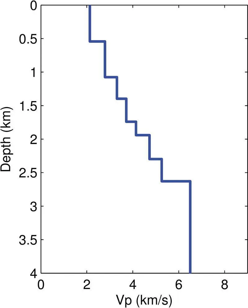
Figure 4.3 P‐wave velocity model for the Kimberlina site.

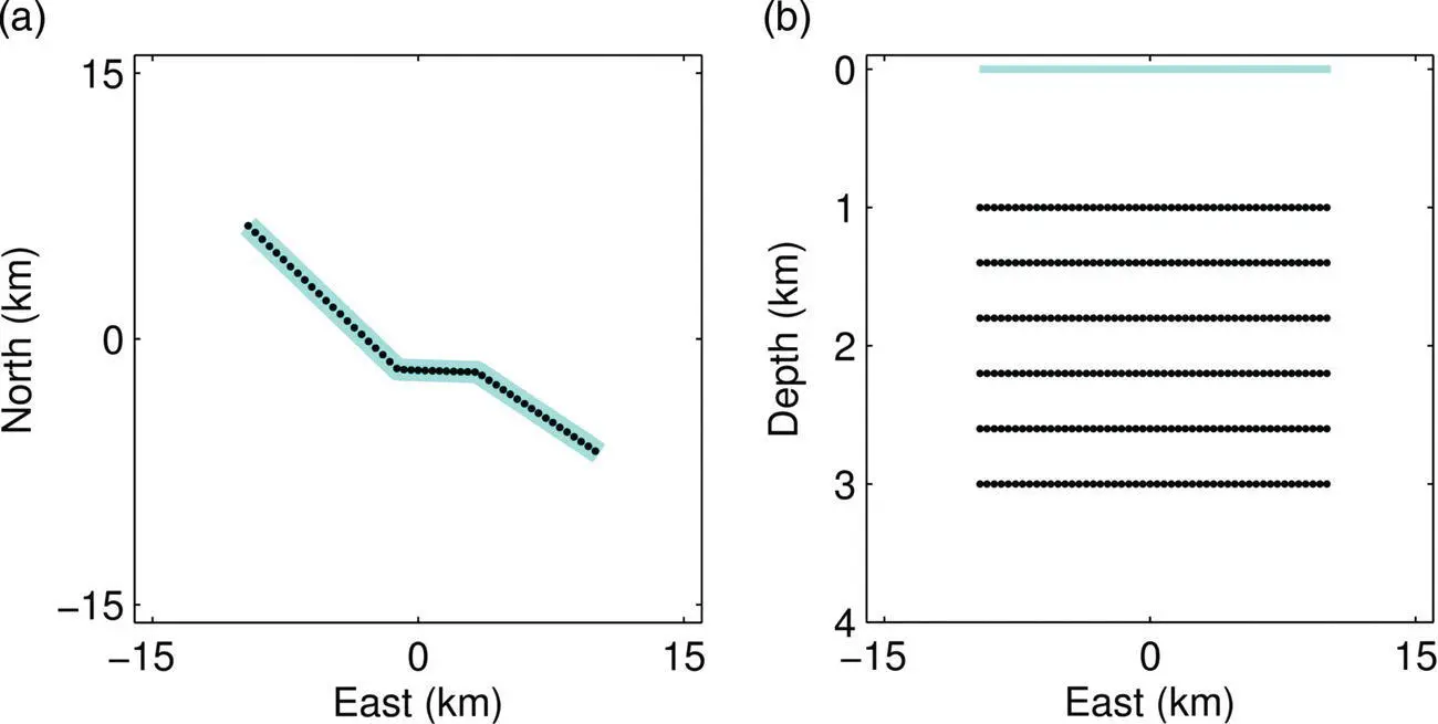
Figure 4.4 The true locations of microseismic events (black dots) used in the synthetic study: (a) map view and (b) depth view. The cyan color shows the simplified surface location of a portion of the Pond‐Poso Creek fault.

For each network distribution, we compute synthetic P‐wave and S‐wave arrival times for the true locations of microseismic events ( Fig. 4.4) through ray tracing using the velocity model in Figure 4.3. We add a random Gaussian error with standard deviations of 0.02 s or 0.05 s to the computed travel times (e.g., Kijko, 1977b). We then use these travel times to solve for the locations of the microseismic events assuming that the velocity models are known. We obtain the linearized least‐squares solutions of event locations and origin times using an iterative inversion scheme (Paige & Saunders, 1982). The initial locations (blue dots in Fig. 4.5) are generated by adding a random Gaussian error with a mean of approximately 500 m to the true locations, and can be considered as an initial guess or some preliminary locations. Because microseismic events are clustered, we also use differential travel times between pairs of events in addition to absolute travel times to better locate the events (Waldhauser & Ellsworth, 2000; Zhang & Thurber, 2003). Improved relative locations using differential travel times are useful for studying the geometry of fractures and faults.

The location results obtained using both P‐wave and S‐wave arrival times with a Gaussian time error of 0.02 s are shown as red dots in Figure 4.5. By increasing the total number of seismic stations, the location results improve with varying degrees. For the horizontal direction, the located events all seem to follow well with true locations (the left column (a), (c), (e), (g) of Fig. 4.5). For the vertical direction, the events are poorly constrained by the 4‐station network because of the lack of a station with small epicentral distances ( Fig. 4.5b). The addition of one station at the center greatly improves the depth location accuracy for the events beneath the station ( Fig. 4.5d). Clear improvement in the event depth is also observed when increasing from 5‐station to 9‐station, and then to 16‐station networks. The event location results with the 25‐station, 36‐station, and 49‐station networks do not seem to show significant difference ( Fig. 4.5f and h).

To show the dependence of location results on different input data, we also conduct the same location inversion process using only P‐wave arrival times and a different Gaussian time error (0.05 s). The location results for these different scenarios are similar to the results shown in Figure 4.5in terms of the improvement of event locations with the increase of the total number of seismic stations. Examples of the location results for these different scenarios are shown in Fig. 4.6, which are all for the 25‐station network. Lower travel time error results in better location results ( Fig. 4.6b vs. f and d vs. h). S‐wave arrivals provide important constraint on the event location, particularly the depth ( Fig. 4.6d vs. b and h vs. f).

We quantify the event location accuracy for each seismic network by calculating the mean error of the located events relative to their true locations. The relationship between the location accuracy and the total number of surface seismic stations for different scenarios is shown in Figure 4.7. The horizontal location ( Fig. 4.7a) is generally better constrained than the depth ( Fig. 4.7b). Adding S‐wave arrival times increases the event location accuracy in both the horizontal direction and vertical directions. Comparing the location results with the 4‐station and 5‐station networks, the vertical location accuracy improves greatly while the horizontal location accuracy improves moderately.

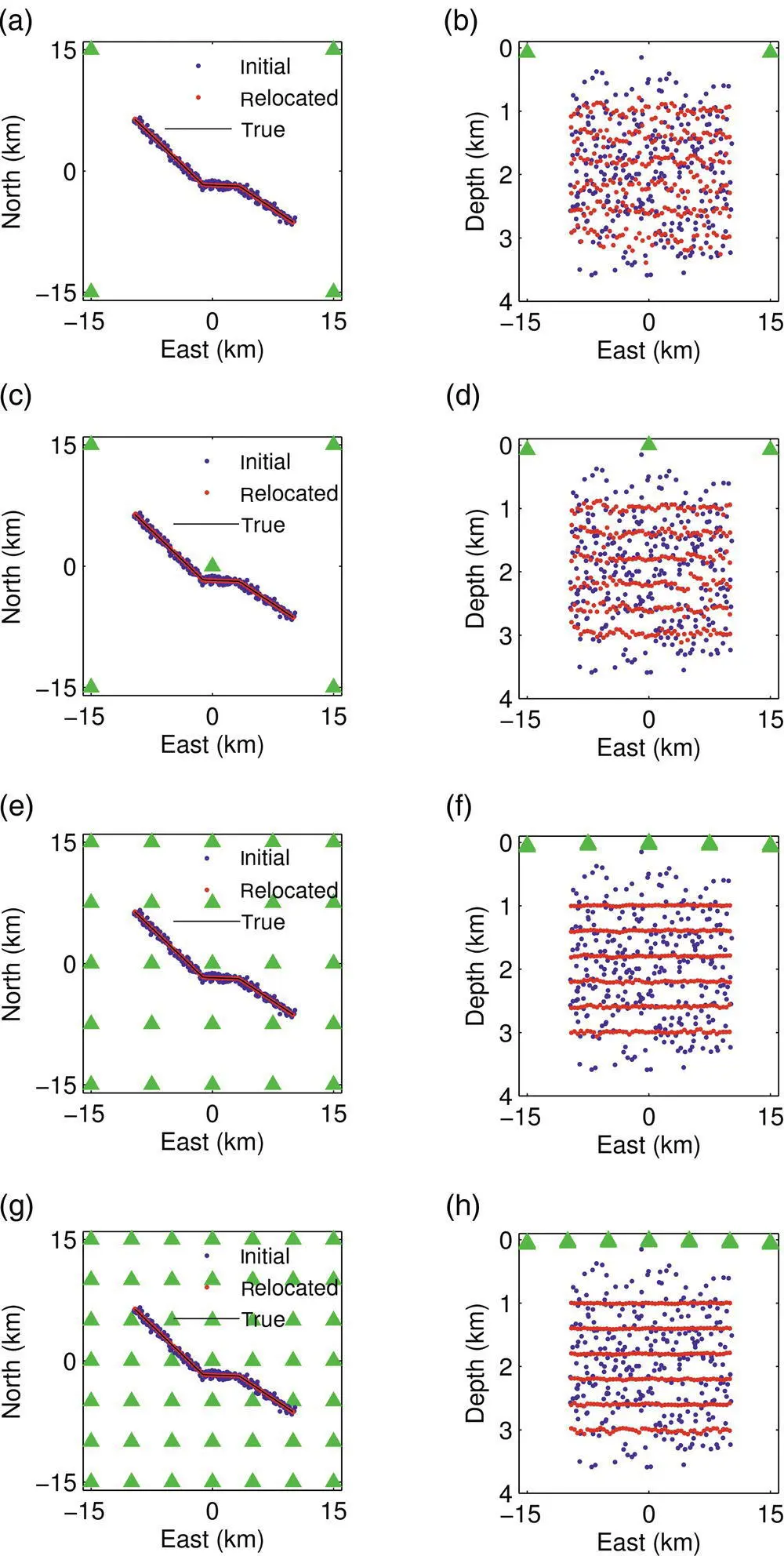
Figure 4.5 The initial (blue dots) and relocated (red dots) microseismic events obtained using different distributions of seismic stations (green triangles) for the synthetic study in Figure 4.4. The left column (a, c, e, g) is map view and the right column (b, d, f, h) is the corresponding depth view. These are the results using both P‐wave and S‐wave arrival times with the 0.02 s noise.

The overall hypocentral location accuracy is shown in Figure 4.7c, which combines both horizontal and vertical location accuracy. For all scenarios, the location accuracy in relation to the number of seismic stations improves rapidly when the seismic network consists of a relatively small numbers of seismic stations. However, further improvement of the location accuracy becomes slower with further increasing the number of seismic stations. To better analyze the relationship between the location accuracy and the total number of seismic stations, we normalize the mean location accuracy for each scenario studied ( Fig. 4.7d). We choose the value obtained with the 5‐station network as the normalization value, because it shows dramatic change compared with the 4‐station network with only one station difference and should be the minimal number of stations required to have effective monitoring for a geometrically satisfactory network distribution shown in this work. The rapid improvement of event location accuracy from using four stations to five stations is also observed for optimal network distributions designed based on a statistical theory (e.g., Kijko, 1977b). The normalized curves between the mean location accuracy and the number of stations for all studied scenarios follow a similar trend. The best trade‐off point can be found by locating the corner of the L‐shaped curves. For the monitoring regions in this example, our result suggests that approximately 20 seismic stations are needed for cost‐effective monitoring.