Geophysical Monitoring for Geologic Carbon Storage

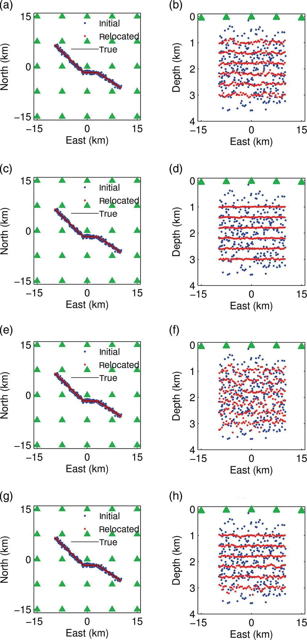
Figure 4.6 The initial (blue dots) and relocated (red dots) microseismic events obtained using 25 seismic stations (green triangles) for the synthetic study in Figure 4.4. The results are for (a‐b) using P‐wave arrival times with the 0.02 s noise, (c‐d) using P‐wave and S‐wave arrival times with the 0.02 s noise, (e‐f) using P‐wave arrival times with the 0.05 s noise, (g‐h) using P‐wave and S‐wave arrival times with the 0.05 s noise.

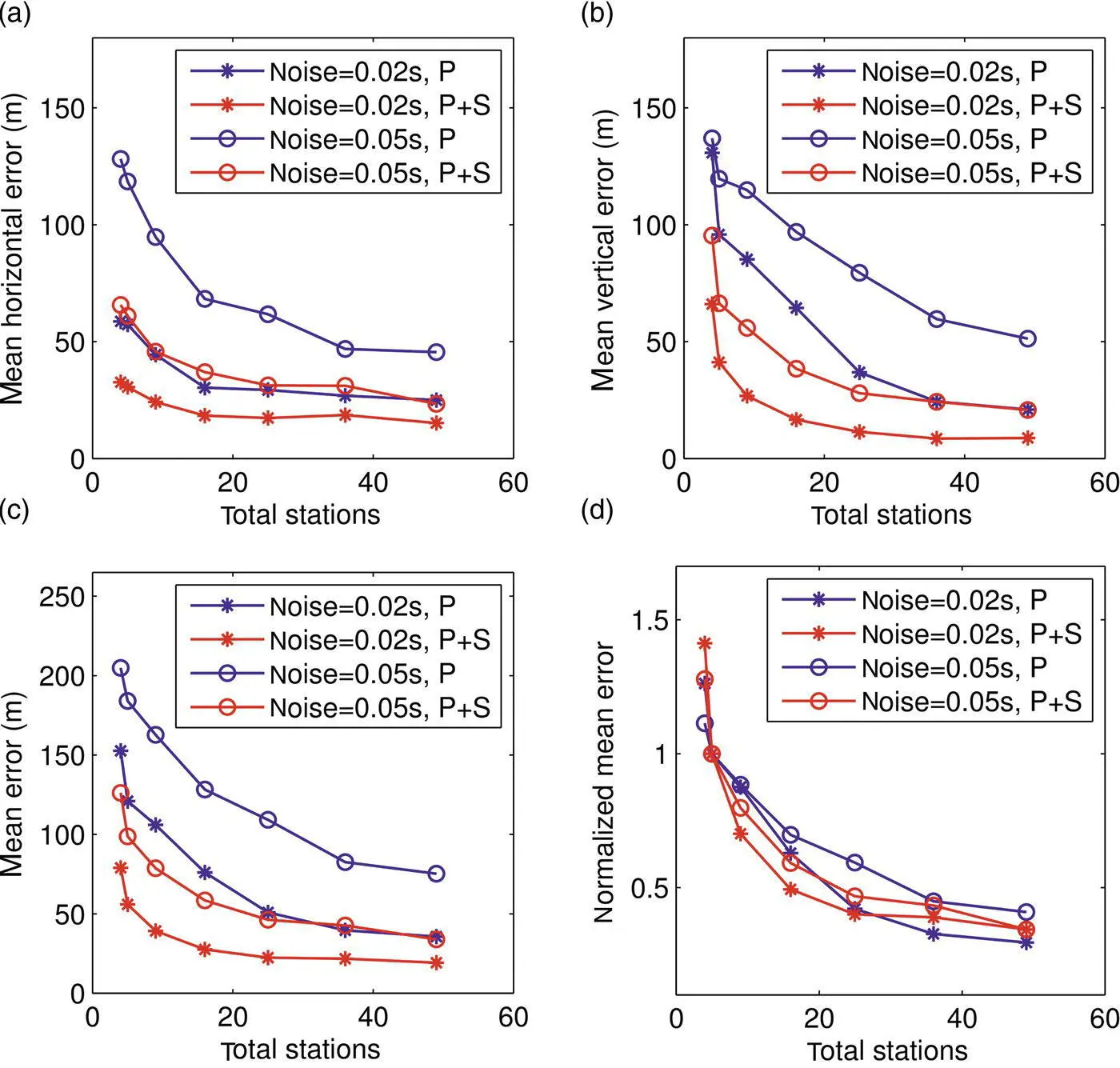
Figure 4.7 Event location accuracy versus the total number of seismic stations: (a) mean horizontal location errors, (b) mean vertical location errors, (c) mean location errors, (d) mean location errors normalized relative to the error obtained with five seismic stations. Blue lines represent results obtained using P‐wave arrival times with different noise levels, red lines represent results obtained using both P‐wave and S‐wave arrival times with different noise levels.

The results shown in Figure 4.7are for regularly distributed seismic networks. We also study irregularly distributed seismic networks to confirm that the results in Figure 4.7are also approximately applicable to irregularly distributed seismic networks as long as the network has a reasonable geometry with adequate azimuthal and distance coverage. We take the 25‐station seismic network as an example. We create an irregularly distributed network by perturbing the regularly spaced network with random distances. We generate 10 randomly distributed 25‐station seismic networks, and Figure 4.8shows two of them as an example. The mean location accuracy obtained with these 10 irregularly distributed 25‐station networks is similar to the value obtained with regularly distributed 25‐station networks ( Fig. 4.9). For the specific monitoring regions in this demonstration example, we determine that approximately 20 stations with geometrically satisfactory distribution can achieve the best trade‐off between the cost and the event location accuracy. It should be noted, though, in this work, we only consider the square distribution around the fault for simplicity. This kind of square distribution covers a wide area, and can be useful for regions where seismic events may also occur on some unknown hidden fractures or faults around the focus fault. If the focus fault is long, an elongate distribution of seismic network surrounding the fault should be preferable.

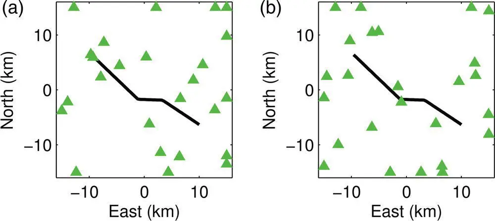
Figure 4.8 (a,b) Two examples of the irregularly distributed 25 seismic stations (green triangles). The Black line shows the simplified surface location of a portion of the Pond‐Poso Creek fault.

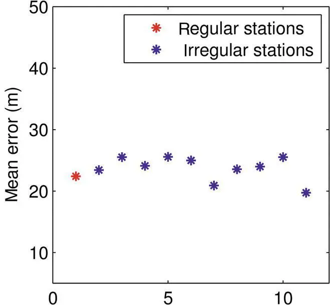
Figure 4.9 Comparison between mean event location accuracy for regularly spaced 25 seismic stations (red dot) and irregularly spaced 25 seismic stations (blue dots). Ten different layouts of irregularly spaced 25 seismic stations are studied. The mean event location accuracy with irregularly spaced seismic stations is similar to the one obtained with regularly spaced seismic stations.

For the case with borehole geophones, similar steps as above for surface seismic networks can be applied to obtain the optimal design of a borehole geophone array. For demonstration, we consider a synthetic case with target microseismic events within the reservoir, at depths between 2.2 km and 2.5 km and within a horizontal region of 2 km. We place a vertical geophone string above the center of the target monitoring region of microseismic events, at depths between 0.2 km and 2.1 km ( Fig. 4.10). We consider regularly spaced geophones along the geophone string. We fix the top and bottom locations, and increase the number of geophones from 5 to 10, 20, 30, 40, 50, 60, 70, 80, 90, and 100. For each geophone distribution, we compute synthetic P‐wave and S‐wave arrival times for the true locations of microseismic events ( Fig. 4.10) using the velocity model in Figure 4.3. We add a random Gaussian error with standard deviations of 0.02 s to the computed travel times. We then use these travel times to solve for the locations of the microseismic events assuming that the velocity models are known. The initial event locations (blue dots in Fig. 4.11) are generated by adding a random Gaussian error with a mean distance of approximately 100 m to the true locations. The final event locations are obtained using the same method described in section 4.3for optimal design of a seismic surface array. Examples of the borehole geophone distribution and final event locations are shown in Figure 4.11.

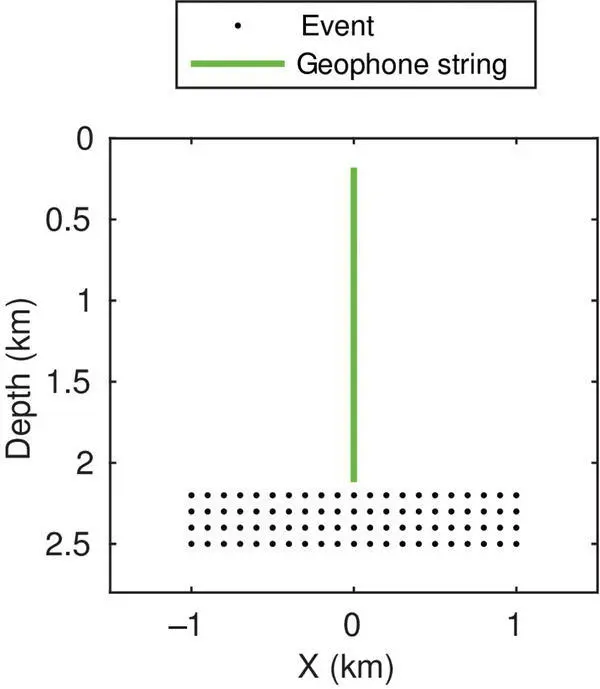
Figure 4.10 The true locations of microseismic events (black dots) used for optimal design of a borehole geophone array.

We quantify the event location accuracy for each geophone distribution by calculating the mean accuracy of located events relative to their true locations. The relationship between the location accuracy and the total number of geophones for different scenarios is shown in Figure 4.12. We see that the event location accuracy does not change much when the number of geophones increases beyond 50. Therefore, 50 would be an optimal number of geophones needed to achieve a good balance between event location accuracy and the cost.

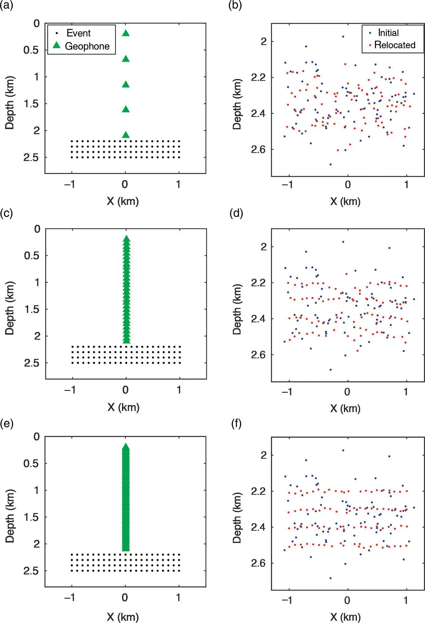
Figure 4.11 The initial (blue dots) and relocated (red dots) microseismic events obtained using different numbers of borehole geophones (green triangles) for the synthetic study in Figure 4.10. The number of geophones shown as examples is 5 (a‐b), 30 (c‐d), and 100 (e‐f).

One assumption we have made in this study is that all seismic stations in the network can record the primary phase arrivals from all events. In reality, only close enough stations can detect useful signals for the seismic events below a certain magnitude. The detection capabilities of stations also depend on the focal mechanism of the events, attenuation structure, and noise level. The synthetic demonstration examples shown in this study can be viewed for only the seismic events that are large enough to be recorded by all seismic stations. Based on the detectability of the smallest seismic events needed to monitor, similar approaches as we describe in this chapter can be applied to different scales.

Different data‐processing procedures, such as single‐component versus multicomponent data processing, single‐station versus array‐signal processing, first arrivals only versus multiple phases, and different location techniques (e.g., Lin & Shearer, 2005; Pesicek et al., 2014), may generate slightly different location results for the same network distribution, but the trade‐off curve between the event location accuracy and the number of seismic stations can still be obtained using the approach described in this chapter.