Geophysical Monitoring for Geologic Carbon Storage

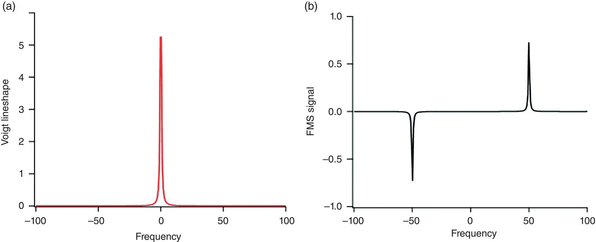
Figure 3.5 (a) A relatively sharp Voigt absorption profile and (b) the corresponding FMS signal plotted as functions of the carrier frequency. The FMS signal was calculated using M = 0.1 and ω m= 50.0.

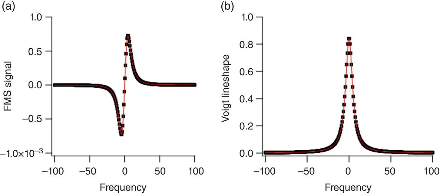
Figure 3.6 Least‐squares fitting of FMS spectra. “Simulated” FMS data (the black squares in plot (a)) were used in a nonlinear least‐squares fit to the FMS signal equation. Voigt parameters (including the absorption coefficient constituents) were taken as the unknowns during regression. The resulting fit is shown as the red line in (a). The Voigt absorption feature calculated from the parameters deduced from the least‐squares fit is shown as a red line in plot (b). The black squares in (b) correspond to the discrete absorption feature used initially to generate the “simulated” FMS data seen in (a).

(3.8)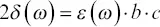

and is used in a nonlinear least squares regression to determine the extinction coefficient ε(ω) as a function of frequency for each feature of interest, while the path length b and concentration c are known. A spectrum for a sample of unknown concentration is then obtained and the previously determined extinction coefficients for the features of interest are used in another least squares regression to determine the concentration, assuming the path length is known. If the path length is not known, the product of concentration and path length can be determined by this regression. A ratio of the regressed parameters then provides the concentration ratio for the two isotopologues. A numerical example of such a regression scheme is highlighted in Figure 3.6.

Figure 3.7contains the FM spectra collected with the in situ instrument discussed above for (a) 12C 16O 2and (b) 13C 16O 2. All of the FMS instruments built at LANL were designed to be research instruments that are capable of probing multiple absorption features as depicted in Figure 3.7.

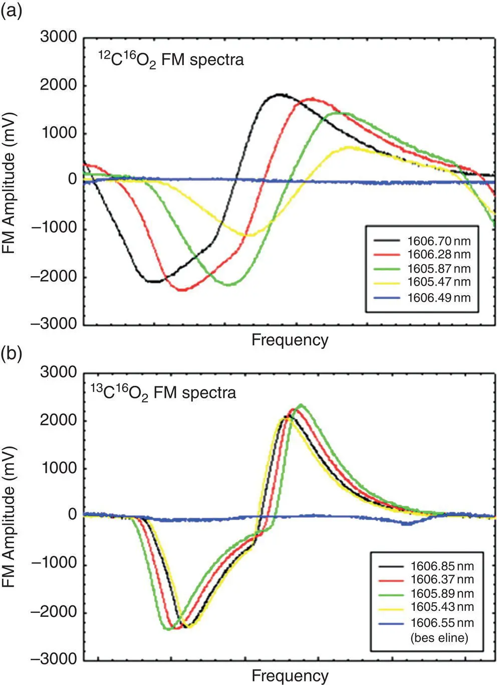
Figure 3.7 The derivative shaped FMS spectrum recorded for several (a) 12C 16O 2and (b) 13C 16O 2transitions. The blue trace in both plots represents the baseline where the laser did not probe CO 2.

The White cell contained ~100 ppm 12C 16O 2and 13C 16O 2, and the laser was scanned across multiple absorption features. Since the CO 2concentration remained constant, the intensity of the FM trace changed with the intensity of the population in each of the rovibrational states. In both experiments, the laser was scanned over the 1,605–1,607 nm range where the population in the 13CO 2states remained relatively constant while the 12CO 2populations were declining. For both experiments, the baseline is depicted in the blue trace at a spectral wavelength that is not absorbed by CO 2and demonstrates the dynamic range available by this method. In principal, only one rovibrational state in 12CO 2and 13CO 2is necessary to calculate an isotope ratio. While these spectra were collected with the in situ instrument with a constant CO 2concentration, one records similar spectra with the remote instrument.

Before conducting field experiments, the in situ instrument is calibrated and validated with 12CO 2and 13CO 2reference standards. This involves flowing reference CO 2through the White cell as it would be used in the field. The CO 2also flows from the White cell and into a LICOR instrument. The FMS trace similar to those in Figure 3.7was recorded and the peak‐to‐peak intensities were extracted from the trace. Calibration curves were generated by plotting the peak‐to‐peak intensities against the CO 2concentration in the White cell as depicted in Figure 3.8. The response over this concentration range is very linear, as expected.

Finally, the instrument was deployed at many locations over many years. By far, most of the data were collected during an annual trip to the Zero Emission Research and Technology (ZERT) field site on the Montana State University campus in Bozeman, Montana (Spangler et al., 2010). The ZERT field site consisted of a horizontally drilled well about 6 ft deep. The ZERT facilitators would use mass flow controllers to deliver a specific amount of CO 2through the well that would leak to the surface simulating a leak from a geologic sequestration site.

The FMS instrument used a small pump to deliver atmospheric gases through a flexible hose into the White cell. The hose was routinely moved from locations over and around the well where leaks were identified. The hose was also placed in locations away from the well as a background. The instrument could collect and analyze a sample every hour autonomously. However, some experiments involved collecting gases in a sealed glass flask for isotope ratio mass spectrometer (IRMS) analysis at LANL. These samples were designed to validate the isotopic ratios recorded in the field. Figure 3.9contains a plot of the FMS results observed against the IRMS results. The plot demonstrates that most of the results are within ± 20% relative agreement while there were a few data points each year that were just outside the ± 20% relative agreement. These data demonstrate that the FMS instrument is capable of making real‐time stable isotope measurements as accurately as the IRMS at these observed concentration levels. These experiments also suggest that stable isotope ratios below ‐15% represent seepage from the reservoir.

Finally, the remote instrument was also deployed at the ZERT field site as depicted in Figure 3.10. The instrument was kept in a Pelican case to protect it from the weather as shown in the bottom of the picture in Figure 3.10. The laser was directed to a corner cube placed 30 m away from the laser source that would direct the laser back to the FMS instrument. The remote FMS instrument would autonomously collect FMS spectra similar to those depicted in Figure 3.7.

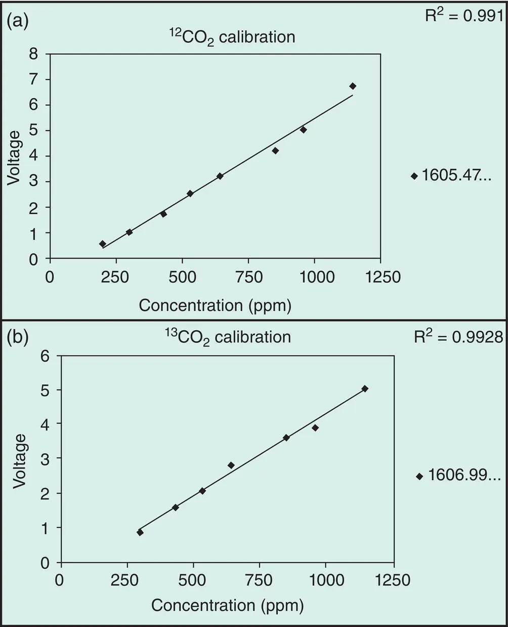
Figure 3.8 A demonstration of the FMS accuracy and sensitivity where calibrated concentrations of (a) 12CO 2and (b) 13CO 2were probed in the White cell.

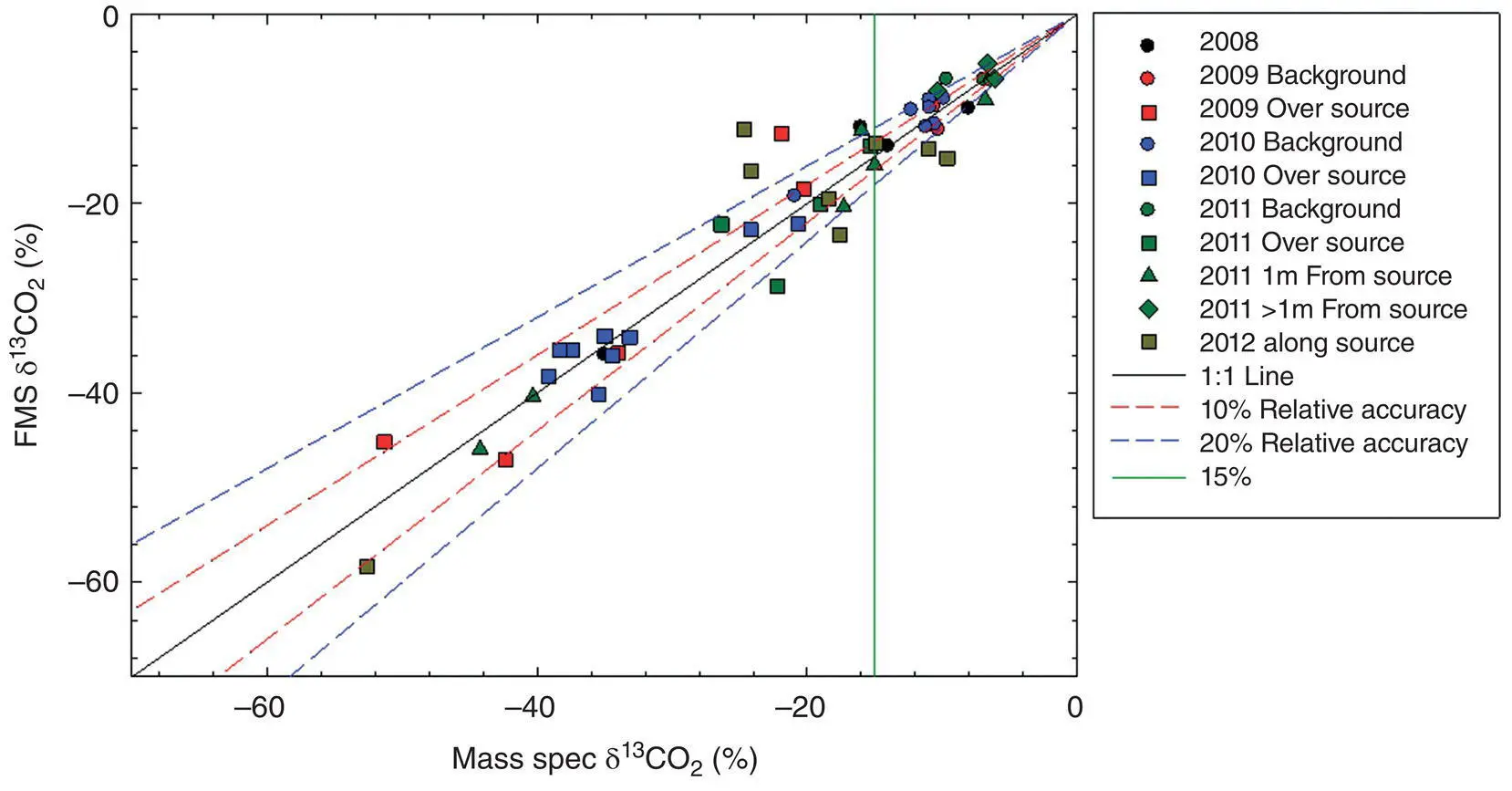
Figure 3.9 A comparison of the FMS stable isotope concentrations measured in the field against IRMS concentrations from collected samples. The different colors represent different years between 2008 and 2012. The shapes represent collections above, around, and away from the source. The black line is the 1:1 line (perfect agreement), while the red and blue dashed lines represent ± 10% and ± 20% relative agreement, respectively.

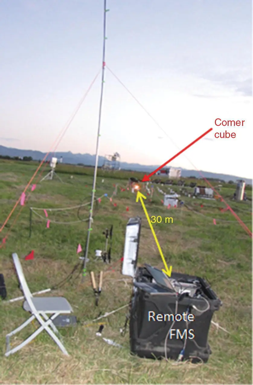
Figure 3.10 The remote FMS instrument was deployed to the ZERT controlled‐release field site. The instrument remained in the weatherproof case and the laser was directed to the corner cube identified by the orange arrow.