Geophysical Monitoring for Geologic Carbon Storage

An FMS LIDAR‐capable instrument fundamentally can accomplish all of the requirements discussed in the introduction. A LIDAR instrument capable of stable isotope sensitivity would distinguish natural CO 2sources from CO 2seepage to the surface and would have some capability to locate the source with the ranging capability.

The development of field deployable FMS instruments started with the construction of an in situ instrument similar to the one depicted in Figure 3.3. The instrument uses a New Focus tunable diode laser (TDL) that scans over the 1,604–1,609 nm CO 2absorption band. A Stanford Research Systems DS345 function generator was used to directly modulate the TDL at 2 GHz. The laser is fiber optically coupled to an Infrared Analysis, Inc., 8 m long multipass White cell. Air samples containing CO 2are pumped into the White cell for analysis. The laser beam exits the White cell, is launched into a second optical fiber that directs the laser into a New Focus detector. The output of the director is filtered and amplified with a Stanford Research Systems SR560 before being recorded on a PC.

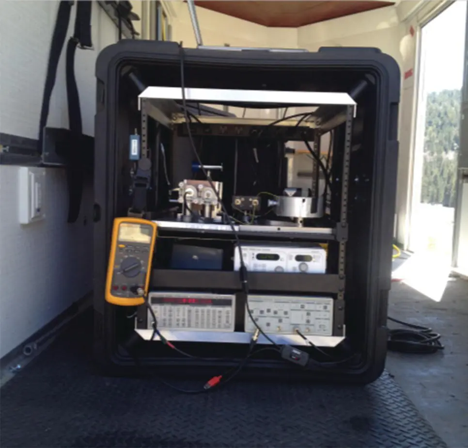
Figure 3.3 The in situ FMS instrument built at Los Alamos National Laboratory enclosed in a weatherproof case for field deployment.

An open‐path remote instrument was developed using the same optical system discussed for the in situ system above. The same model New Focus TDL was fiber optically coupled to a 5x beam expander used to collimate an enlarged beam. The modulated beam was directed to a retroreflector placed up to hundreds of meters away from the beam expander. The returned laser beam was collected with a second beam expander, coupled to a second optical fiber and onto the New Focus detector.

Superimposing a periodic (sinusoidal) frequency upon a light wave having a base, or carrier, frequency of ω oresults in a frequency modulated wave described by

(3.2)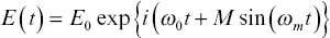

where E ois the electric field amplitude, t is time, M is the modulation index (or strength) of the imposed periodic variation, and ω mis the frequency of the periodic “dithering” frequency. When passed through a sample, both absorption and dispersion of the wave occur. To account for these, convention is to use a complex valued frequency‐dependent transmission function, T(ω) , defined as

(3.3)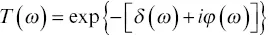

where δ accounts for the absorption, ϕ accounts for the dispersion, and ω is the instantaneous frequency, which depends on ω o, ω m, M , and t . As defined, δ embodies the product of path length, extinction coefficient, and concentration. The wave exiting the sample is then

(3.4)

where the transmission function serves as a susceptibility. The intensity of the wave leaving the sample, I(t) , is given by the electric field E(t) times its complex conjugate. This leads to (Supplee et al., 1994)

(3.5)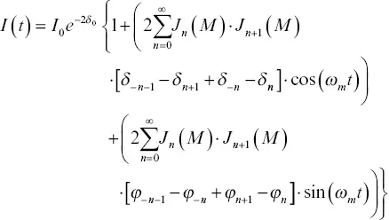

where I ois the incident wave intensity, J(M) denotes a Bessel function of the first kind, and the summation index n corresponds to the various sidebands. For weak absorption at the carrier frequency, δ ois essentially zero and the resulting FMS signal then depends only on the dithering frequency ω m. Thus, by a judicious choice of dithering frequency, one can, in principle, avoid much of the system noise and obtain high signal‐to‐noise ratios using FMS. Exploiting this basic attribute of FMS has resulted in ppb‐level sensitivity (Votsmeier et al., 1999; Werle et al.1993; Reid et al., 1980) and excellent signal‐to‐noise data (Dubinsky et al., 1998; Song & Jung, 2003). Note that the absorption terms are out of phase, or in quadrature, with the dispersion terms, that is, the absorption is associated with the cosine and the dispersion with the sine. In practice, a phase angle between the incident and transmitted light beams is typically observed at the detector. This is due to the change in light propagation speed through the sample and the fact that the path lengths between source and detector usually differ for the two beams. Consequently, the argument of the sine and cosine terms ( ω m t ) is often replaced by that phase angle, which we denote as θ . Experimentally, the phase angles can be adjusted (i.e., matched) so that θ = 0 will give a pure absorption FMS signal.

FMS is often implemented using a small modulation index (i.e., small M ) and where only the n = 0 sidebands are important. Under such conditions, the equation for the FMS signal intensity can be simplified considerably to give the often‐used working equation

(3.6)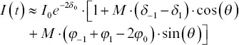

Note, for completeness, that when phase matching is employed (such that θ . =0 ), and the M goes to zero limit is taken, one arrives at

(3.7)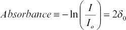

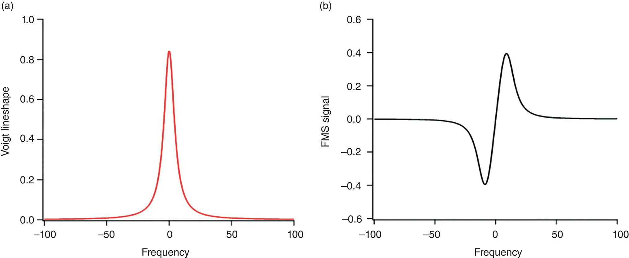
Figure 3.4 An example of (a) Voigt absorption profile and (b) the corresponding FMS signal plotted as functions of the carrier frequency. The FMS signal was calculated using M = 10.0 and ω m= 1.0.

which is essentially Beer's law for absorption at the carrier frequency ω o(the factor of two here results from taking the product of the transmission function and its complex conjugate).

Consider an absorption event represented by a Voigt absorption profile (assumed to be centered at zero for convenience). Figure 3.4shows such a Voigt profile along with the corresponding (numerically calculated) FMS signal for the case of a relatively small dithering frequency. As another numerical example, consider the case of a sharp absorption feature and a relatively large dithering frequency, which is displayed in Figure 3.5. Depending on the relative sharpness of the absorption feature and the magnitude of the dithering frequency, a wide range of qualitatively and quantitatively distinct FMS signals can be realized, some considerably more complicated than the examples displayed above (Bjorklund & Levenson, 1983).

Application of FMS to species that differ only in their isotopic composition can rely on identifying absorption features that are shifted in frequency and hence become distinct. The absorption associated with each distinct feature then provides concentration information for that species. For illustrative purposes, one means of implementing FMS to detect isotopologues of a given species (e.g., light and heavy CO 2or light and heavy CH 4) is outlined. First, calibration spectra for the two distinct features are obtained using known concentrations of each isotopologue. Next, the absorption coefficient is broken into its conventional components, namely,