Manuel Pastor - Computational Geomechanics

(1.10b)

Those not familiar with soil mechanics may find the following hypothetical experiment illustrative. A block of porous, sponge‐like rubber is immersed in a fluid to which an increase in pressure of Δ p is applied as shown in Figure 1.4. If the pores are connected to the fluid, the volumetric strain will be negligible as the solid components of the sponge rubber are virtually incompressible.

If, on the other hand, the block is first encased in a membrane and the interior is allowed to drain freely, then again a purely volumetric strain will be realized but now of a much larger magnitude.

The facts mentioned above were established by the very early experiments of Fillunger (1915) and it is surprising that so much discussion of “area coefficients” has since been necessary.

From the preceding discussion, it is clear that if the material is subject to a simultaneous change of total stress Δ σ and of the total pore pressure Δ p , the resulting strain can always be written incrementally in tensorial notation as

(1.11a)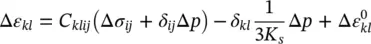

or in vectoral notation

(1.11b)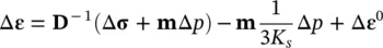

with

(11.11c)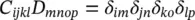

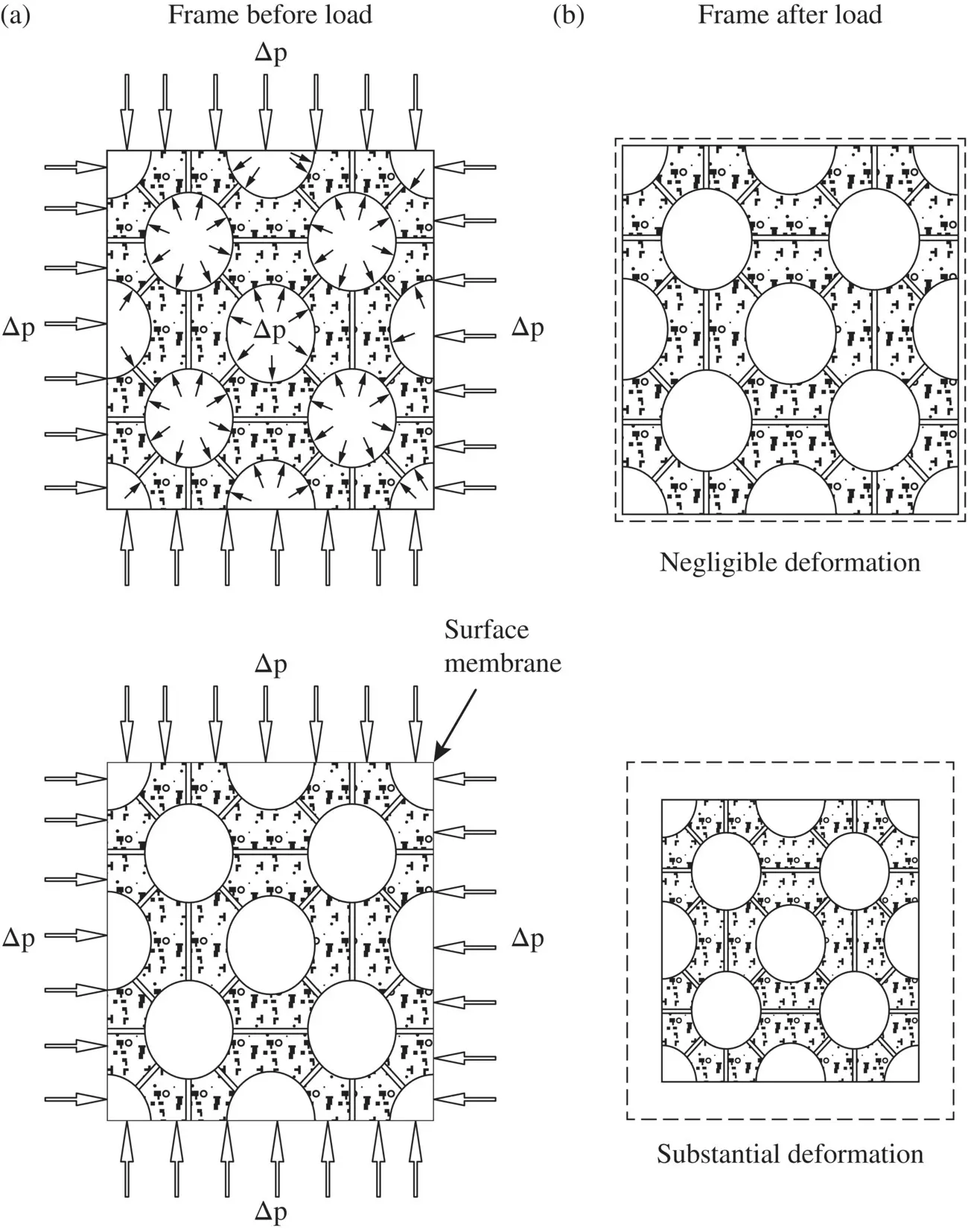
Figure 1.4 A porous material subject to external hydrostatic pressure increases Δ p, and (a) internal pressure increment Δ p; (b) internal pressure increment of zero.

The last term in (1.11a)and (1.11b), Δ ε 0, is simply the increment of an initial strain such as may be caused by temperature changes, etc., while the penultimate term is the strain due to the grain compression already mentioned, viz. Equation (1.10). Dis a tangent matrix of the solid skeleton implied by the constitutive relation with corresponding compliance coefficient matrix D −1= C. These, of course, could be matrices of constants, if linear elastic behavior is assumed, but generally will be defined by an appropriate nonlinear relationship of the type which we shall discuss in Chapter 4and this behavior can be established by fully drained ( p = 0) tests.

Although the effects of skeleton deformation due to the effective stress defined by ( 1.6) with n w= 1 have been simply added to the uniform volumetric compression, the principle of superposition requiring linear behavior is not invoked and in this book, we shall almost exclusively be concerned with nonlinear, irreversible, elastoplastic and elastoviscoplastic responses of the skeleton which, however, we assume incremental properties.

For assessment of the strength of the saturated material, the effective stress previously defined with n w= 1 is sufficient. However, we note that the deformation relation of (1.11) can always be rewritten incorporating the small compressive deformation of the particles as (1.12).

It is more logical at this step to replace the finite increment by an infinitesimal one and to invert the relations in (1.11) writing these as

(1.12a)

or

(1.12b)

where a new “effective” stress, σ″ , is defined. In the above

(1.13a)

or

(1.13b)

and the new form eliminates the need for separate determination of the volumetric strain component. Noting that, in three dimensions,

or

we can write

(1.14a)

or simply

Alternatively, in tensorial form, the same result is obtained as

(1.14b)

and

For isotropic materials, we note that,

(1.15a)

which is the tangential bulk modulus of an isotropic elastic material with λ and μ being the Lamé’s constants. Thus we can write

(1.15b)

The reader should note that in (1.12), we have written the definition of the effective stress increment which can, of course, be used in a non‐incremental state as

(1.16a)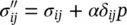

or

(1.16b)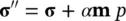

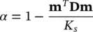
assuming that all the stresses and pore pressure started from a zero initial state (for example, material exposed to air is taken as under zero pressure). The above definition corresponds to that of the effective stress used by Biot (1941) but is somewhat more simply derived. In the above, α is a factor that becomes close to unity when the bulk modulus K sof the grains is much larger than that of the whole material. In such a case, we can write, of course

(1.17a)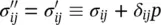

or

(1.17b)