Isotopic Constraints on Earth System Processes

In a multi‐component system, the diffusive flux J i(moles m 2/s) of component i is given by:

(2.3)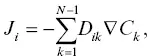

where D ik(m 2/s) is the multicomponent diffusion matrix and C kis the concentration of component k in volume‐normalized units. The off‐diagonal terms in the diffusion matrix represent diffusive coupling between components, which may be kinetic (the diffusing species have a stoichiometry that differs from the stoichiometry of the chosen components of the system) or thermodynamic (the flux of one component influences the activity or concentration of another). The full diffusion matrix has been determined for only a few simplified silicate liquid systems (Chakraborty et al., 1995; Kress & Ghiorso, 1993; Liang, 2010; Liang & Davis, 2002; Liang et al., 1996; Mungall et al., 1998; Oishi et al., 1982; Richter et al., 1998; Sugawara et al., 1977; Wakabayashi & Oishi, 1978; Watkins et al., 2014) as well as some basaltic liquids (Guo & Zhang, 2016, 2018; Kress & Ghiorso, 1995). The full diffusion matrix is not known for either phonolite or rhyolite. Even if it were known, it would be composition dependent in the mixing region between the two liquids, and at present there is no general way of dealing with such a complex diffusion problem. Therefore, it is not practical to use a multicomponent diffusion model for describing the fluxes in the rhyolite‐phonlite diffusion couple, and a simplified approach must be employed.

The effective binary diffusion (EBD) model (Cooper, 1968) is often used in applications where the goal is to infer timescales of magmatic processes in complex systems (cf. Zhang, 2010). In this framework, the flux of component i is proportional to its own concentration gradient:

(2.4)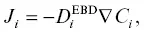

where D i EBDis the effective binary diffusion coefficient (EBDC) and is sensitive to melt composition and the direction of diffusion in composition space (Liang, 2010; Zhang, 2010).

There are a number of shortcomings of the EBD model, but the main one for our purposes is that it cannot describe uphill diffusion. This led Zhang (1993) to propose a modified EBD model based on the concept of elemental partitioning between two liquids of different composition. The Zhang model treats the diffusive flux of a component as being proportional to an activity gradient instead of a concentration gradient (following Zhang’s notation, we drop the subscript i to make the expressions easier to read):

(2.5)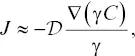

where γ is the activity coefficient and is the “intrinsic effective binary diffusivity.” At equilibrium, the activity ( a = γC ) is uniform but there may still be concentration gradients, as would be the case for the interface between two phases or two immiscible liquids. Note that = when γ is constant. For simplicity, we adopt the simplest version of the Zhang model and assume that 1/ γ is a linear function of SiO 2concentration and is independent of the concentration of all other components. Alternatively, one might assume that the activity has an exponential dependence on SiO 2concentration (e.g., Richter, 1993), but this ultimately yields similar profiles and does not change our overall conclusions (see Supplemental Information 2.A). Regardless, for a given transient profile of SiO 2, there exists an associated hypothetical “quasi‐equilibrium” profile for the equilibrium concentration of the component of interest, C e, that scales with 1/ γ as well as the concentration of SiO 2. Assuming that diffusion of SiO 2can be characterized by a concentration‐independent EBD, D b, and that diffusion of SiO 2does not reach either end of the diffusion couple, the “equilibrium” concentration profile for C eis an error function:

(2.6)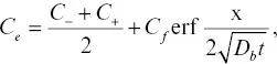

where C −and C +are the initial concentrations at x < 0 and x > 0 for the diffusion couple and C fis the difference in the equilibrium concentration between the two liquids, as depicted in Fig. 2.5. The parameter C fcan be positive or negative, depending on whether the component preferentially partitions into the high‐silica or low‐silica liquid. A large C fimplies strong preference for one liquid versus the other. If C f= 0, the model reverts back to the simplified EBD model. Replacing γ with 1/ C ein equation 2.5yields

(2.7)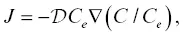

which leads to the one‐dimensional diffusion equation (Eq. 9a in Zhang, 1993):

(2.8)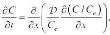

where the units of concentration may be in weight percent if density can be assumed to be constant. The reason for the approximation symbol in equation 2.5is that Zhang (1993) uses equation 2.8to calculate concentration profiles and then calculates activity profiles from the relation a = kC / C e, where k is the proportionality constant between C eand 1/ γ . A point that was nuanced by Zhang (1993) is that equations 2.5and 2.7are not equivalent, but rather are scaled by a factor k , which can be determined from the constraint that a = C at x = 0 (interface).

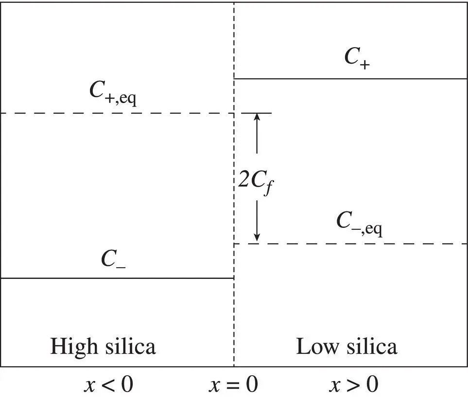
Figure 2.5 The Zhang model and its parameters are based on the concept of elemental partitioning in an SiO 2gradient. The initial concentration distribution is C +for x > 0 and C −for x < 0. At equilibrium, the concentration contrast may be reversed (depending on the sign of C f) such that C +, eq for x < 0 and C −, eq for x > 0.

The Zhang (1993) model deviates significantly from the EBD model when the component of interest diffuses significantly faster than SiO 2. In this situation, which is common in silicate liquids, the component of interest will not reach homogeneity quickly, but rather, will partition along the compositional continuum between the high‐ and low‐silica liquids and reach compositional homogeneity only as fast as SiO 2diffuses.