Maintenance, Reliability and Troubleshooting in Rotating Machinery

2 A trend where the slope of the cumulative failures versus time sharply increases in July of 2016, indicating a decreasing failure rate (shown as “Decreasing” in Figure 2.5).

3 A trend where the slope of the cumulative failures versus time decreases in July 2016, indicating an increasing failure rate (shown as “Improving” in Figure 2.5).

When readers study a reliability growth plot, they are able to discern if pump reliability is constant, deteriorating or improving. Other insights that a reliability growth plot provide are when a change in reliability occurred, and if the change in reliability was sudden or gradual. In this case, seen in Figure 2.5, we note the deteriorating case indicating that something changed after July 2016. We should look for changes in operating procedures, repair methods, processing rates, etc., to explain changes in pump reliability. Persistent changes in pump reliability may represent some sort of major change affecting your pump or pumps, while a data blip could simply be measurement error, or some sporadic factor, such as a plant upset.

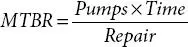
The next reliability plot we will cover is the mean time between repairs (MTBF) trend plot ( Figure 2.6). MTBF is a simple calculation that provides insight into the mechanical reliability of a single or a group of pumps, which is calculated as follow:

Let’s go through an example of how we can evaluate the change in the MTBF of a large population. Let’s assume you have 1,000 pumps in your facility and that in year #1 you repaired 375 pumps and that in year #2 you repaired 300 pumps.

The average MTBF for year #1 is:

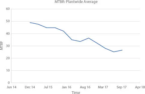
Figure 2.6 A hypothetical trend plot of the plantwide mean time between repairs (MTBF).

The average MTBF for year #2 is:

These data show a 25% improvement in the mean time between pump failures from year #1 to year #2.

Instead of continuously calculating the MTBF and reporting a single number to management, we can plot the moving average trend of a population’s MTBF. This type of plot can be used to keep an eye on a single or large population of process machines. A moving average MTBF plot is constructed by calculating then plotting the calculated MTBF from the data from the previous month, quarter, or year. Plotting the MTBF data in this way tends to smooth out the data and simplifies the analysis. By inspection, we can see that the MTBF of a hypothetical pump population in Figure 2.6is gradually deteriorating. Your next step might be to examine the individual trends of each of your process units to see if they are all deteriorating or if there are some poorly performing unit populations forcing the overall plantwide reliability down.

MTBF: Readers should keep in mind that the MTBF metric is a global metric and only provides limited information about a given machine population. As you drill down to the equipment levels, more advanced analyses, such as Weibull analyses, may be warranted to examine the failure data and to better understand the nature of the failures.

I have briefly covered a few machinery reliability analysis tools that I have personally used to analyze spared machines during my career. The data used to create these metrics are readily available and can easily be organized and then analyzed using Excel or similar software applications. The concise visual results can then be quickly interpreted by your colleagues and management.

As mentioned earlier, critical machines tend to be regarded differently by management than spared machines because:

Owners are usually more concerned about the availability of critical machines than their maintenance costs.

There is a much smaller set of critical failure data than spared machine failure data.

Production losses tend to dominate the economics of critical machines.

For these reasons, availability, trends of process outages, production loss trends, Pareto downtime causes (machinery, exchangers, controls, etc.), and root causes are often used to track the reliability of critical machinery.

Availability, also known as uptime, calculates what percentage of the time a piece of equipment was actually performed (or was able to perform if called upon by the site). It is an essential metric for measuring the overall effectiveness of an asset. If a machine’s availability falls below a tolerable level, then the site must investigate the reason(s) why and develop a plan to improve it.

Normally, a tangible asset tends to lose its availability performance as it is used over time. Technicians can improve the asset’s availability by undertaking essential maintenance tasks. However, when availability drops below a specific threshold, the asset’s performance will not improve unless it is upgraded or replaced. There are several ways to calculate availability. The first is as follows:

An alternative means of determining availability is as follows:

Here is a simple example using the uptime/downtime method: A critical machine ran for 700 hours in a given month. During that month, the asset also had 12 hours of unplanned downtime because of a breakdown, and 8 hours of downtime for weekly PMs, which equals 20 hours of total downtime. Therefore 700 uptime hours + 20 downtime hours = 720 total hours. Using these numbers, we can determine the availability for the month is equal to 700/(700+20) = 97.22%.

Tracking availability can help identify opportunities for improvements by identifying problematic equipment. The typical availability benchmark is above 95% for most assets. However, it can differ depending on how necessary the equipment is to your operations.

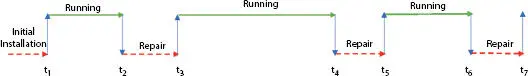
Figure 2.7 Hypothetical machine history. Green (solid) arrows indicate machine is running and red (dashed) arrows indicate machine is down for maintenance.

Without historical lifecycle data, we cannot make objective decisions about machines. To determine a critical machine’s availability, we need to know how long it ran between outages and how long it took to make repairs. Therefore, we need a database that can capture life cycle events for all your critical machines.

Consider the life cycle of the hypothetical machine seen in Figure 2.7. At t 1the machine is started for the first time. The machine runs reliably from time t 1to t 2and fails. The machine is repaired from time t 2to t 3and then restarted at time t 3. The machine runs from t 3to t 4and fails. The machine is repaired from time t 4to t 5and then restarted. The machine runs from t 5to t 6and fails at time t 6. The machine is repaired from time t 6to t 7and then restarted.