Feitian Zhang - Mobile Robots

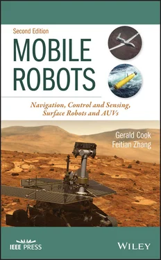
1 Cover

2 Preface

3 About the Authors

4 Introduction

5 1 Kinematic Models for Mobile Robots1.1 Introduction 1.2 Vehicles with Front‐Wheel Steering 1.3 Vehicles with Differential‐Drive Steering Exercises References

6 2 Mobile Robot Control2.1 Introduction 2.2 Front‐Wheel Steered Vehicle, Heading Control 2.3 Front‐Wheel Steered Vehicle, Speed Control 2.4 Heading and Speed Control for the Differential‐Drive Robot 2.5 Reference Trajectory and Incremental Control, Front‐Wheel Steered Robot 2.6 Heading Control of Front‐Wheel Steered Robot Using the Nonlinear Model 2.7 Computed Control for Heading and Velocity, Front‐Wheel Steered Robot 2.8 Heading Control of Differential‐Drive Robot Using the Nonlinear Model 2.9 Computed Control for Heading and Velocity, Differential‐Drive Robot 2.10 Steering Control Along a Path Using a Local Coordinate Frame 2.11 Optimal Steering of Front‐Wheel Steered Vehicle 2.12 Optimal Steering of Front‐Wheel Steered Vehicle, Free Final Heading Angle Exercises References

7 3 Robot Attitude 3.1 Introduction 3.2 Definition of Yaw, Pitch, and Roll 3.3 Rotation Matrix for Yaw 3.4 Rotation Matrix for Pitch 3.5 Rotation Matrix for Roll 3.6 General Rotation Matrix 3.7 Homogeneous Transformation 3.8 Rotating a Vector Exercises References

8 4 Robot Navigation4.1 Introduction 4.2 Coordinate Systems 4.3 Earth‐Centered Earth‐Fixed Coordinate System 4.4 Associated Coordinate Systems 4.5 Universal Transverse Mercator Coordinate System 4.6 Global Positioning System 4.7 Computing Receiver Location Using GPS, Numerical Methods 4.8 Array of GPS Antennas 4.9 Gimbaled Inertial Navigation Systems 4.10 Strap‐Down Inertial Navigation Systems 4.11 Dead Reckoning or Deduced Reckoning 4.12 Inclinometer/Compass Exercises References

9 5 Application of Kalman Filtering5.1 Introduction 5.2 Estimating a Fixed Quantity Using Batch Processing 5.3 Estimating a Fixed Quantity Using Recursive Processing 5.4 Estimating the State of a Dynamic System Recursively 5.5 Estimating the State of a Nonlinear System via the Extended Kalman Filter Exercises References

10 6 Remote Sensing 6.1 Introduction 6.2 Camera‐Type Sensors 6.3 Stereo Vision 6.4 Radar Sensing: Synthetic Aperture Radar 6.5 Pointing of Range Sensor at Detected Object 6.6 Detection Sensor in Scanning Mode Exercises References

11 7 Target Tracking Including Multiple Targets with Multiple Sensors 7.1 Introduction 7.2 Regions of Confidence for Sensors 7.3 Model of Target Location 7.4 Inventory of Detected Targets Exercises References

12 8 Obstacle Mapping and Its Application to Robot Navigation8.1 Introduction 8.2 Sensors for Obstacle Detection and Geo‐Registration 8.3 Dead Reckoning Navigation 8.4 Use of Previously Detected Obstacles for Navigation 8.5 Simultaneous Corrections of Coordinates of Detected Obstacles and of the Robot Exercises References

13 9 Operating a Robotic Manipulator9.1 Introduction 9.2 Forward Kinematic Equations 9.3 Path Specification in Joint Space 9.4 Inverse Kinematic Equations 9.5 Path Specification in Cartesian Space 9.6 Velocity Relationships 9.7 Forces and Torques Exercises References

14 10 Remote Sensing via UAVs10.1 Introduction 10.2 Mounting of Sensors 10.3 Resolution of Sensors 10.4 Precision of Vehicle Instrumentation 10.5 Overall Geo‐Registration Precision Exercise References

15 11 Dynamics Modeling of AUVs11.1 Introduction 11.2 Motivation 11.3 Full Dynamic Model 11.4 Hydrodynamic Model 11.5 Reduced‐Order Longitudinal Dynamics 11.6 Computation of Steady Gliding Path in the Longitudinal Plane 11.7 Scaling Analysis 11.8 Spiraling Dynamics 11.9 Computation of Spiral Path Exercises References

16 12 Control of AUVs12.1 Introduction 12.2 Longitudinal Gliding Stabilization 12.3 Yaw Angle Regulation 12.4 Spiral Path Tracking Exercises References

17 Appendix A: Demonstrations of Undergraduate Student Robotic ProjectsDemonstrations of Undergraduate Student Robotic ProjectsA.1 Introduction A.2 Demonstration of the GEONAVOD Robot A.3 Demonstration of the Automatic Balancing Robotic Bicycle (ABRB)

18 Index

19 End User License Agreement

1 Chapter 4Table 4.1 Convergence of coordinates as a function of iteration number. Newto...Table 4.2 Convergence of coordinates as a function of iteration number. Perfo...

2 Chapter 7Table 7.1 Typical values of gamma from chi‐square tables.Table 7.2 Inventory with a single target in the field of view of sensor.Table 7.3 Inventory with two targets in the field of view of sensor.

3 Chapter 8Table 8.1a First set of covariances for above example.Table 8.1b Estimates of obstacle location and robot location before and after...Table 8.2a Second set of covariances for above example.Table 8.2b Estimates of obstacle location and robot location before and after...

4 Chapter 11Table 11.1 Computed steady gliding path under different values of the center ...Table 11.2 Computed steady gliding path under different values of the center ...Table 11.3 Computed steady gliding path for the scaled models of the larger w...Table 11.4 Parameters of the miniature underwater glider used in the steady‐s...Table 11.5 Computed spiraling steady states through Newton's method.

5 Chapter 12Table 12.1 System parameters used in simulation.

1 Chapter 1 Figure 1.1 Schematic diagram of the front‐wheel steered robot. Figure 1.2 Schematic diagram of differential‐drive robot.

2 Chapter 2 Figure 2.1 α versus ( ψ des− ψ ) for α = K ( ψ des− ψ ... Figure 2.2 α versus ( ψ des− ψ ) for α = sign( ψ des... Figure 2.3 ( ψ des− ψ ) versus time for α = sign( ψ des− Figure 2.4 α versus time for α = sign( ψ des− ψ ). Figure 2.5 α versus ( ψ des− ψ ) for the control algorithm of e... Figure 2.6 α versus time for ψ (0) = 0 and ψ des= π /2, K ... Figure 2.7 ψ versus time for ψ (0) = 0 and ψ des= π /2, K ... Figure 2.8 (a) Steering angle α versus time. (b) Desired heading and ac... Figure 2.9 Construction for evaluating travel time. Figure 2.10 Path being followed by mobile robot and definition of local coor... Figure 2.11 Simulation A illustrating the heuristic steering control strateg... Figure 2.12 Simulation B illustrating the heuristic steering control strateg...Figure 2.13 Block diagram of the closed‐loop steering system in local coordi...Figure 2.14 Block diagram in original coordinates for mobile robot following...Figure 2.15 Mobile robot recovering from 2 m error while tracking a straight...Figure 2.16 Mobile robot recovering from 2 m error while tracking a segment ...Figure 2.17 Mobile robot recovering from 2 m error while tracking a gently s...Figure 2.18 (a) Trajectory in x – y space. (b) λ ψversus time. (c) α ...Figure 2.19 (a) Trajectory in x – y space. (b) λ ψversus time. (c) α ...Figure 2.20 (a) Trajectory in x – y space. (b) λ ψversus time. (c) α ...Figure 2.21 (a) Trajectory in x – y space. (b) λ ψversus time. (c) α ...Figure 2.22 (a) Trajectory in x – y space. (b) λ ψversus time. (c) α ...Figure 2.23 Trajectory in x – y space for Example 8.Figure 2.24 Trajectory in x – y space for Example 9.Figure 2.25 Trajectory in x – y space.