Feitian Zhang - Mobile Robots

From time to time, it will be convenient to interpret speed expressed in various units. For this reason the following equalities are presented.

Another common type of steering used for mobile robots is differential‐drive steering illustrated in Figure 1.2. Here the wheels on one side of the robot are controlled independently of the wheels on the other side. By coordinating the two different speeds, one can cause the robot to spin in place, move in a straight line, move in a circular path, or follow any prescribed trajectory.

The equations of motion for the robot steered via differential wheel speeds are now derived. Let R represent the instantaneous radius of curvature of the robot trajectory. The width of the vehicle, i.e., spacing between the wheels, is designated as W . From geometrical considerations we have:

(1.7a)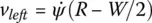

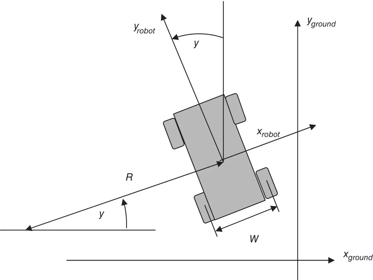
Figure 1.2 Schematic diagram of differential‐drive robot.

and

(1.7b)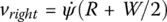

Now subtracting the two above equations yields

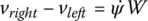
so we obtain for the angular rate of the robot

(1.8)

Solving for the instantaneous radius of curvature, we have:

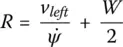
or

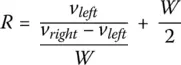
or finally

(1.9)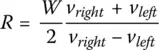

This results in the expression for velocity along the robot's longitudinal axis:

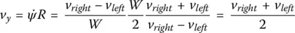
In summary, the equations of motion in robot coordinates are:

(1.10a)

(1.10b)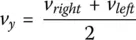

and

(1.10c)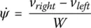

If we convert to earth coordinates these become:

(1.11a)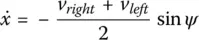

(1.11b)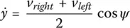

and

(1.11c)

As we did in the case for the robot with front‐wheel steering, we may wish to account for the fact that velocities cannot change instantaneously. Thus, we would introduce as the control variables the velocity rates:

(1.12a)

and

(1.12b)

The system of equations for this kinematic model is now fifth order.

Again we can use the Euler integration method for obtaining a discrete‐time model for this system of nonlinear equations,

(1.13a)

(1.13b)

(1.13c)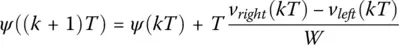

(1.13d)

and

(1.13e)

More sophisticated and more accurate methods for obtaining discrete‐time models exist; however, this Euler model may be quite useful if the sampling interval is set sufficiently small. These discrete‐time models may be used for system analysis, controller design, estimator design, and system simulation. More complex models for mobile robots could also include pitch, roll, and vertical motion.

1 A front‐wheel steered robot is to turn to the left with a radius of curvature equal to 20 m. The robot is 1 m wide and 2 m long. What should the steering angle be?

2 A differential wheel steered robot is to turn to the left with a radius of curvature equal to 20 m and is to travel at 1 m/s. The width is 1 m and the length is 2 m. What should be the velocities of the right side and the left side?

3 Using the discrete‐time model presented, perform a digital simulation of the front‐wheel steered robot using a steering angle of 45°, a length of 1.5 m, and a speed of 2.778 m/s. Experiment with the sample interval, T and find the maximum allowable value that yields consistent results.

4 Develop a digital simulation for the steered wheel robot modeled in Chapter 1. Assume that the width from wheel to wheel is 1 m and that the length, axle to axle is 2 m. A sequence of speeds and steering angles will be inputs. Include limits in your model so that steering angle will not exceed ±45° regardless of the command. Simulate the robot for straight line motion and for motion when the steering angle is held constant at 45° and then constant at −45°. Simulate several seconds of motion. Use the Euler formula for integration and experiment with the sampling interval. Then use a sampling interval of 0.1 s and see if this sampling interval yields correct results. Plot x vs. t, y vs. t, heading vs. t, and y vs. x.

5 Develop a digital simulation for the differential drive robot, modeled in Chapter 1. Assume that the width from wheel to wheel is 1 m and that the length, axle to axle is 2 m. A sequence of right side speeds and left side speeds will be the inputs. Simulate for straight line motion and for motion when the right side speed is 10% above the average speed (right speed + left speed)/2 and the left side speed is 10% below the average speed. Simulate several seconds of motion. Use the Euler formula for integration and experiment with the sampling interval. Then use a sampling interval of 0.1 s and see if this sampling interval yields correct results. Plot x vs. t, y vs. t, heading vs. t, and y vs. x.