Bhisham C. Gupta - Statistics and Probability with Applications for Engineers and Scientists Using MINITAB, R and JMP

where are the weights attached to , respectively. Thus, her GPA is given by

The mode of a data set is the value that occurs most frequently. The mode is the least used measure of centrality. When items are produced via mass production, for example, clothes of certain sizes or rods of certain lengths, the modal value is of great interest. Note that in any data set, there may be no mode, or conversely, there may be multiple modes. We denote the mode of a data set by .

Example 2.5.6(Finding a mode) Find the mode for the following data set:

3, 8, 5, 6, 10, 17, 19, 20, 3, 2, 11

Solution:In the data set of this example, each value occurs once except 3, which occurs twice. Thus, the mode for this set is

Example 2.5.7(Data set with no mode) Find the mode for the following data set:

1, 7, 19, 23, 11, 12, 1, 12, 19, 7, 11, 23

Solution:Note that in this data set, each value occurs twice. Thus, this data set does not have any mode.

Example 2.5.8(Tri‐modal data set) Find the mode for the following data set:

5, 7, 12, 13, 14, 21, 7, 21, 23, 26, 5

Solution:In this data set, values 5, 7, and 21 occur twice, and the rest of the values occur only once. Thus, in this example, there are three modes, that is,

These examples show that there is no mathematical relationship among the mean, mode, and median in the sense that if we know any one or two of these measures (i.e., mean, median, or mode), then we cannot find the missing measure(s) without using the data values. However, the values of mean, mode, and median do provide important information about the type or shape of the frequency distribution of the data. Although the shape of the frequency distribution of a data set could be of any type, in practice, the most frequently encountered distributions are the three types shown in Figure 2.5.1. The location of the measures of centrality as shown in Figure 2.5.1provides the information about the shape of the frequency distribution of a given data.

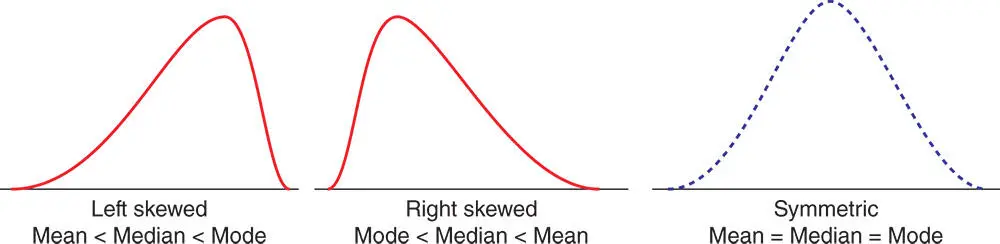
Figure 2.5.1Frequency distributions showing the shape and location of measures of centrality.

A data set is symmetric when the values in the data set that lie equidistant from the mean, on either side, occur with equal frequency.

A data set is left‐skewed when values in the data set that are greater than the median occur with relatively higher frequency than those values that are smaller than the median. The values smaller than the median are scattered to the left far from the median.

A data set is right‐skewed when values in the data set that are smaller than the median occur with relatively higher frequency than those values that are greater than the median. The values greater than the median are scattered to the right far from the median.

In the previous section, we discussed measures of centrality, which provide information about the location of the center of frequency distributions of the data sets under consideration. For example, consider the frequency distribution curves shown in Figure 2.5.2. Measures of central tendency do not portray the whole picture of any data set. For example, it can be seen in Figure 2.5.2that the two frequency distributions have the same mean, median, and mode. Interestingly, however, the two distributions are very different. The major difference is in the variation among the values associated with each distribution. It is important, then, for us to know about the variation among the values of the data set. Information about variation is provided by measures known as measures of dispersion . In this section, we study three measures of dispersion: range , variance , and standard deviation .

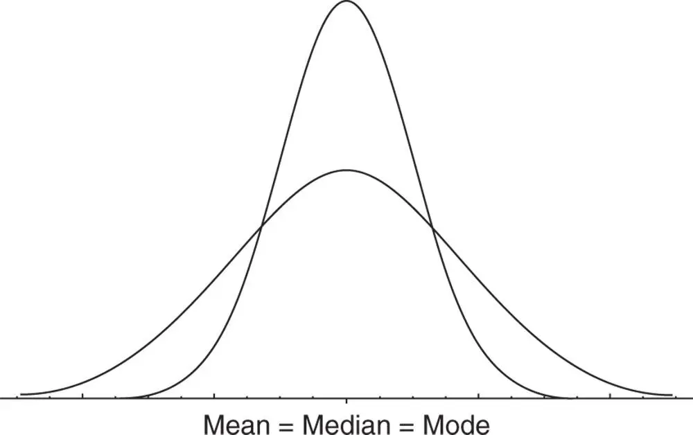
Figure 2.5.2Two frequency distribution curves with equal mean, median, and mode values.

The range of a data set is the easiest measure of dispersion to calculate. Range is defined as

(2.5.5)

The range is not an efficient measure of dispersion because it takes into consideration only the largest and the smallest values and none of the remaining observations. For example, if a data set has 100 distinct observations, it uses only two observations and ignores the remaining 98 observations. As a rule of thumb, if the data set contains 10 or fewer observations, the range is considered a reasonably good measure of dispersion. For data sets containing more than 10 observations, the range is not considered to be an efficient measure of dispersion.

Example 2.5.9(Tensile strength) The following data gives the tensile strength (in psi) of a sample of certain material submitted for inspection. Find the range for this data set:

8538.24, 8450.16, 8494.27, 8317.34, 8443.99, 8368.04, 8368.94, 8424.41, 8427.34, 8517.64

Solution:The largest and the smallest values in the data set are 8538.24 and 8317.34, respectively. Therefore, the range for this data set is

One of the most interesting pieces of information associated with any data is how the values in the data set vary from one another. Of course, the range can give us some idea of variability. Unfortunately, the range does not help us understand centrality. To better understand variability, we rely on more powerful indicators such as the variance , which is a value that focuses on how far the observations within a data set deviate from their mean.

For example, if the values in a data set are , and the sample average is , then are the deviations from the sample average. It is then natural to find the sum of these deviations and to argue that if this sum is large, the values differ too much from each other, but if this sum is small, they do not differ from each other too much. Unfortunately, this argument does not hold, since, as is easily proved, the sum of these deviations is always zero, no matter how much the values in the data set differ. This is true because some of the deviations are positive and some are negative. To avoid the fact that this summation is zero, we can square these deviations and then take their sum. The variance is then the average value of the sum of the squared deviations from . If the data set represents a population, then the deviations are taken from the population mean . Thus, the population variance , denoted by (read as sigma squared), is defined as